In part 1 of this series I showed how to use Power Query to extract Extended Event data generated by SSAS. Having done that, I now want to show the first (I hope of many) examples of how this data can be used for performance tuning: analysing activity in the Storage Engine, the part of SSAS that reads data from disk and aggregates it up.

I won’t go into the technical details of how I’ve used Power Query to crunch this data; you can download the sample workbook here and see for yourself. There’s nothing particularly complex going on. In brief, what I’ve done is the following:

• Called the function shown in part 1 to get the raw Extended Event data
• Filtered that data so that only the Query End, Query Subcube Verbose and Progress Report End events are left
• Calculated the start time of each event relative to the start time of the earliest recorded event, to make plotting these events on a waterfall chart possible
• Built an Excel report, including various Power Pivot measures, some normal slicers to make it easy to filter the data, some disconnected slicers for filtering so you only see events that started within a given time range, and a PivotChart showing the waterfall chart (since Excel doesn’t support this type of chart natively, I’ve used this technique to reproduce a waterfall chart with a stacked bar chart)

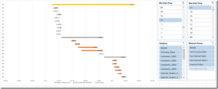
Here’s an example screenshot of the result, showing Storage Engine activity for a single query:

Though it’s hard to see the details at this resolution, the yellow line is the Query End event associated with the query, the grey lines are the Query Subcube Verbose events associated with the query, and the brown lines are the Progress Report events associated with each Query Subcube Verbose event.

What could this be used for? Here are some ideas:

• Looking for times when there are a lot of queries running simultaneously – and which, as a result, may be performing poorly.
• Looking for long-running Query Subcube Verbose and Progress Report End events which could be optimised by the creation of aggregations.
• Visualising the amount of parallelism inside the Storage Engine, in particular the number of Progress Report End events that are running in parallel. This would be very interesting for queries using distinct count measures when you are testing different ways of partitioning your measure group.
• Highlighting situations where calculations are being evaluated in cell-by-cell mode. When this happens you typically see a very large number of Query Subcube Verbose events being fired off within a query.

I’d like to stress once again that the object of this exercise is not to show off a ‘finished’ tool, but to show how Power Query, Power Pivot and Excel can be used for self-service analysis of this data. This workbook is just a starting point: if you wanted to use this on your own data it’s extremely likely you’d need to change the Power Query queries, the Power Pivot model and the report itself. Hopefully, though, this workbook will save you a lot of time if you do need to understand what’s going on in the Storage Engine when you run an MDX query.

Last year I blogged about how to introduce a delay between web service requests in M code. Since then a new function has been added to Power Query which makes this a lot easier: Function.InvokeAfter(). This function doesn’t seem to be documented anywhere apart from the Power Query language reference (downloadable from here); the signature is as follows:

Function.InvokeAfter(function as function, delay as duration) as any

It invokes a function after waiting for a given amount of time. Here’s a simple example of how it can be used that declares a function which returns the current date/time as text, then calls it twice with a five second delay in between:

let
    GetTimeAsText = ()=> DateTime.ToText(DateTime.LocalNow()),
    Output = GetTimeAsText() & " "
                   & Function.InvokeAfter(GetTimeAsText, #duration(0,0,0,5))
in
    Output

The output of this query (at the time of writing) is:

28/04/2015 23:06:38 28/04/2015 23:06:43

One thing that did confuse me a bit was the fact that Function.InvokeAfter() doesn’t allow you to pass a list of arguments for the function you’re invoking like Function.Invoke(). The nice people at Microsoft helped me out with this though, and here’s a slightly more complicated example showing how to use Function.InvokeAfter() with a function that appends “Hello “ to a person’s name:

let
    SayHello = (personname as text) as text => "Hello " & personname,
    Output = Function.InvokeAfter(()=>SayHello("Chris"), #duration(0,0,0,5))
in
    Output

I saw an interesting post the other day on the Power Query Technet forum which showed how the List.Buffer() function could be used to improve calculation performance. This is something I’d seen hinted at in other places so I thought it was worth a bit of investigation.

Consider the following query:

let
    //Connect to SQL Server
    Source = Sql.Database("localhost", "adventure works dw"),
    //Get first 2000 rows from FactInternetSales
    dbo_FactInternetSales = Table.FirstN(
          Source{[Schema="dbo",Item="FactInternetSales"]}[Data],
          2000),
    //Remove unwanted columns
    RemoveColumns = Table.SelectColumns(
          dbo_FactInternetSales,
          {"SalesOrderLineNumber", "SalesOrderNumber","SalesAmount"}),
    //Get sorted list of values from SalesAmount column
    RankValues = List.Sort(RemoveColumns[SalesAmount], Order.Descending),
    //Calculate ranks
    AddRankColumn = Table.AddColumn(RemoveColumns , "Rank",
          each List.PositionOf(RankValues,[SalesAmount])+1)
in
    AddRankColumn

It gets the first 2000 rows from the FactInternetSales table in the Adventure Works DW database, removes most of the columns, and adds a custom column that shows the rank of the current row based on its Sales Amount.

On my laptop it takes around 35 seconds to run this query – pretty slow, in my opinion, given the amount of data in this table.

However, using the List.Buffer() function in the RankValues step like so:

let
    //Connect to SQL Server
    Source = Sql.Database("localhost", "adventure works dw"),
    //Get first 2000 rows from FactInternetSales
    dbo_FactInternetSales = Table.FirstN(
          Source{[Schema="dbo",Item="FactInternetSales"]}[Data],
          2000),
    //Remove unwanted columns
    RemoveColumns = Table.SelectColumns(
          dbo_FactInternetSales,
          {"SalesOrderLineNumber", "SalesOrderNumber","SalesAmount"}),
    //Get sorted list of values from SalesAmount column
    //And buffer them!
    RankValues = List.Buffer(List.Sort(RemoveColumns[SalesAmount], Order.Descending)),
    //Calculate ranks
    AddRankColumn = Table.AddColumn(RemoveColumns , "Rank",
          each List.PositionOf(RankValues,[SalesAmount])+1)
in
    AddRankColumn

Makes the query run in just 2 seconds. The List.Buffer() function stores the sorted list of values used to calculate the rank in memory which means it will only be evaluated once; in the original query it seems as though this step and those before it are being evaluated multiple times. Curt Hagenlocher’s comment (on this thread) on what List.Buffer() does for a similar calculation is telling:

The reason for this is that M is both functional and lazy, so unless we buffer the output of List.Select, we’re really just building a query that needs to be evaluated over and over. This is similar to the Enumerable functions in LINQ, if you’re familiar with those.

Table.Buffer() and Binary.Buffer() functions also exist, and do similar things.

A few other points to make:

• This is not necessarily the optimal way to calculate ranks in Power Query – it’s just an example of how List.Buffer() can be used.
• In the first query above, query folding is not taking place. If it had been it’s likely that performance would have been better. Since using List.Buffer() explicitly prevents query folding from taking place, it could make performance worse rather than better because of this in many cases.
• I’m 100% certain you’ll get much better performance for a rank calculation by loading the table to the Excel Data Model/Power Pivot and writing the calculation in DAX. You should only really do calculations like this in Power Query if they are needed for other transformations in your query.

Quite often, in Power Query, you want to ‘nest’ calculations and transformations – apply them not across the whole table, but repeat the same calculation or transformation across multiple groups of rows within that table. Let me give you an example…

Take the following input table:

Imagine you wanted to add a column showing the rank of each row by Sales. In Power Query you would just need to:

1. Load the data
2. Sort the table in descending order by Sales
3. Add an index column starting at 1, which is the rank

You would end up with the following output:

…and here’s the M code, all of which is generated by the UI:

let
    Source = Excel.CurrentWorkbook(){[Name="Sales"]}[Content],
    #"Sorted Rows" = Table.Sort(Source,{{"Sales", Order.Descending}}),
    #"Added Index" = Table.AddIndexColumn(#"Sorted Rows", "Rank", 1, 1)
in
    #"Added Index"

Now imagine you wanted to rank Sales within each month. That’s to say you want to apply the same steps as shown in the previous query but for each month individually to get an output like this:

One way to tackle this, and problems like it, is to do the following. First, do a Group By on the column you want to repeat the calculation over, in this case Month, and use the All Rows aggregation operation. This will result in a table with one row for each month and a column containing nested tables, as shown below:

Each one of these tables contains the rows from the original table for the month.

You can then take your original transformation and turn it into a function, either in a separate query or as a step in your current query. Here’s an example of how the query above can be turned into a function that takes a table and returns a table with a rank column added:

(tabletorank as table) as table =>
     let
      SortRows = Table.Sort(tabletorank,{{"Sales", Order.Descending}}),
      AddIndex = Table.AddIndexColumn(SortRows, "Rank", 1, 1)
     in
      AddIndex

Next, you need to pass each nested table to this function. You could do that in a calculated column, but the most elegant way I think is by using the Table.TransformColumns() function which takes a function and applies it to every value in a column (see here for another example of how to use it).

Finally, you get the final output by clicking on the Expand icon in the AllRows column and then choosing to expand all the columns in the nested table except the ones you originally grouped on:

Here’s the full M code:

let
    //Get data from Excel
    Source = Excel.CurrentWorkbook(){[Name="Sales"]}[Content],
    //Group by Month
    Grouped = Table.Group(Source, {"Month"}, {{"AllRows", each _, type table}}),
    //Declare a function that adds a Rank column to a table
    RankFunction = (tabletorank as table) as table =>
     let
      SortRows = Table.Sort(tabletorank,{{"Sales", Order.Descending}}),
      AddIndex = Table.AddIndexColumn(SortRows, "Rank", 1, 1)
     in
      AddIndex,
    //Apply that function to the AllRows column
    AddedRank = Table.TransformColumns(Grouped, {"AllRows", each RankFunction(_)}),
    //Expand the tables in the AllRows column again
    ExpandAgain = Table.ExpandTableColumn(AddedRank, "AllRows",
       {"Product", "Sales", "Rank"}, {"Product", "Sales", "Rank"})
in
    ExpandAgain

You can download the example workbook here.

This pattern could also be applied to other types of calculation that need to be nested, for example running totals or shares.

Power Query is great for filtering data before it gets loaded into Excel, and when you do that you often need to provide a friendly way for end users to choose what data gets loaded exactly. I showed a number of different techniques for doing this last week at SQLBits but here’s my favourite: using Excel slicers.

Using the Adventure Works DW database in SQL Server as an example, imagine you wanted to load only only rows for a particular date or set of dates from the FactInternetSales table. The first step to doing this is to create a query that gets all of the data from the DimDate table (the date dimension you want to use for the filtering). Here’s the code for that query – there’s nothing interesting happening here, all I’m doing is removing unnecessary columns and renaming those that are left:

let
    Source = Sql.Database("localhost", "adventure works dw"),
    dbo_DimDate = Source{[Schema="dbo",Item="DimDate"]}[Data],
    #"Removed Other Columns" = Table.SelectColumns(dbo_DimDate,
        {"DateKey", "FullDateAlternateKey", "EnglishDayNameOfWeek", 
        "EnglishMonthName", "CalendarYear"}),
    #"Renamed Columns" = Table.RenameColumns(#"Removed Other Columns",{
        {"FullDateAlternateKey", "Date"}, {"EnglishDayNameOfWeek", "Day"}, 
        {"EnglishMonthName", "Month"}, {"CalendarYear", "Year"}})
in
    #"Renamed Columns"

Here’s what the output looks like:

Call this query Date and then load it to a table on a worksheet. Once you’ve done that you can create Excel slicers on that table (slicers can be created on tables as well as PivotTables in Excel 2013 but not in Excel 2010) by clicking inside it and then clicking the Slicer button on the Insert tab of the Excel ribbon:

Creating three slicers on the Day, Month and Year columns allows you to filter the table like so:

The idea here is to use the filtered rows from this table as parameters to control what is loaded from the FactInternetSales table. However, if you try to use Power Query to load data from an Excel table that has any kind of filter applied to it, you’ll find that you get all of the rows from that table. Luckily there is a way to determine whether a row in a table is visible or not and I found it in this article written by Excel MVP Charley Kyd:

http://www.exceluser.com/formulas/visible-column-in-excel-tables.htm

You have to create a new calculated column on the table in the worksheet with the following formula:

=(AGGREGATE(3,5,[@DateKey])>0)+0

This calculated column returns 1 on a row when it is visible, 0 when it is hidden by a filter. You can then load the table back into Power Query, and when you do you can then filter the table in your new query so that it only returns the rows where the Visible column contains 1 – that’s to say, the rows that are visible in Excel. Here’s the code for this second query, called SelectedDates:

let
    Source = Excel.CurrentWorkbook(){[Name="Date"]}[Content],
    #"Filtered Rows" = Table.SelectRows(Source, each ([Visible] = 1)),
    #"Removed Columns" = Table.RemoveColumns(#"Filtered Rows",{"Visible"})
in
    #"Removed Columns"

This query should not be loaded to the Excel Data Model or to the worksheet.

Next, you must use this table to filter the data from the FactInternetSales table. Here’s the code for a query that does that:

let
    Source = Sql.Database("localhost", "adventure works dw"),
    dbo_FactInternetSales = Source{[Schema="dbo",Item="FactInternetSales"]}[Data],
    #"Removed Other Columns" = Table.SelectColumns(dbo_FactInternetSales,
        {"ProductKey", "OrderDateKey", "CustomerKey", "SalesOrderNumber", 
        "SalesOrderLineNumber", "SalesAmount", "TaxAmt"}),
    Merge = Table.NestedJoin(#"Removed Other Columns",{"OrderDateKey"},
        SelectedDates,{"DateKey"},"NewColumn",JoinKind.Inner),
    #"Removed Columns" = Table.RemoveColumns(Merge,
        {"ProductKey", "OrderDateKey", "CustomerKey"}),
    #"Expand NewColumn" = Table.ExpandTableColumn(#"Removed Columns", 
        "NewColumn", {"Date"}, {"Date"}),
    #"Reordered Columns" = Table.ReorderColumns(#"Expand NewColumn",
        {"Date", "SalesOrderNumber", "SalesOrderLineNumber", 
        "SalesAmount", "TaxAmt"}),
    #"Renamed Columns" = Table.RenameColumns(#"Reordered Columns",{
        {"SalesOrderNumber", "Sales Order Number"}, 
        {"SalesOrderLineNumber", "Sales Order Line Number"}, 
        {"SalesAmount", "Sales Amount"}, 
        {"TaxAmt", "Tax Amount"}}),
    #"Changed Type" = Table.TransformColumnTypes(#"Renamed Columns",
        {{"Date", type date}})
in
    #"Changed Type"

Again, most of what this query does is fairly straightforward: removing and renaming columns. The important step where the filtering takes place is called Merge, and here the data from FactInternetSales is joined to the table returned by the SelectedDates query using an inline merge (see here for more details on how to do this):

The output of this query is a table containing rows filtered by the dates selected by the user in the slicers, which can then be loaded to a worksheet:

The last thing to do is to cut the slicers from the worksheet containing the Date table and paste them onto the worksheet containing the Internet Sales table:

You now have a query that displays rows from the FactInternetSales table that are filtered according to the selection made in the slicers. It would be nice if Power Query supported using slicers as a data source direct without using this workaround and you can vote for it to be implemented here.

You can download the sample workbook for this post here.

Following on from my recent post on Power BI and Excel 2016 news, here are some more details about the new BI-related features in the Excel 2016 Preview. Remember that more BI-related features may appear before the release of Excel 2016, and that with Office 365 click-to-run significant new features can appear in between releases, so this is not a definitive list of what Excel 2016 will be able to do at RTM but a snapshot of functionality available as of March 2015 as outlined in this document and which I’ve found from my own investigations. When I find out more, or when new functionality appears, I’ll either update this post or write a new one.

Power Query

Yesterday, in the original version of my post, I mistakenly said that Power Query was a native add-in in Excel 2016: that’s not true, it’s not an add-in at all, it’s native Excel functionality. Indeed you can see that there is no separate Power Query tab any more, and instead there is a Power Query section on the Data tab instead:

Obviously I’m a massive fan of Power Query so I’m biased, but I think this is a great move because it makes all the great Power Query functionality a lot easier to discover. There’s nothing to enable – it’s there by default – although I am a bit worried that users will be confused by having the older Data tab features next to their Power Query equivalents.

There are no new features for Power Query here compared to the latest version for Excel 2013, but that’s what I expected.

Excel Forecasting Functions

I don’t pretend to know anything about forecasting, but I had a brief play with the new Forecast.ETS function and got some reasonable results out of it as seen in the screenshot below:

Slicer Multiselect

There’s a new hammer icon on a slicer, which, when you click it, changes the way selection works. The default behaviour is the same as Excel 2013: every time you click on an item, that item is selected and any previous selection is lost (unless you were holding control or shift to multiselect). However with the hammer icon selected each new click adds the item to the previously selected items. This is meant to make slicers easier to use with a touch-screen.

Time Grouping in PivotTables

Quite a neat feature this, I think. If you have a table in the Excel Data Model that has a column of type date in it, you can add extra calculated columns to that table from within a PivotTable to group by things like Year and Month. For example, here’s a PivotTable I built on a table that contains just dates:

Right-clicking on the field containing the dates and clicking Group brings up the following dialog:

Choosing Years, Quarters and Months creates three extra fields in the PivotTable:

And these fields are implemented as calculated columns in the original table in the Excel Data Model, with DAX definitions as seen here:

Power View on SSAS Multidimensional

At-bloody-last. I haven’t installed SSAS on the VM I’m using for testing Excel 2016, but I assume it just works. Nothing new in Power View yet, by the way.

Power Map data cards

Not sure why this is listed as new in Excel 2016 when it seems to be the same feature that appeared in Excel 2013 Power Map recently:

https://support.office.com/en-za/article/Customize-a-data-card-in-Power-Map-797ab684-82e0-4705-a97f-407e4a576c6e

Power Pivot

There isn’t any obvious new functionality in the Power Pivot window, but it’s clear that the UI in general and the DAX formula editor experience in particular has been improved.

Suggested Relationships

When you use fields from two Excel Data Model tables that have no relationship between them in a PivotTable, you get a prompt to either create new relationships yourself or let Excel detect the relationships:

Renaming Tables and Fields in the Power Pivot window

In Excel 2013 when you renamed tables or fields in the Excel Data Model, any PivotTables that used those objects had them deleted. Now, in Excel 2016, the PivotTable retains the reference to table or field and just displays the new name. What’s even better is that when you create a measure or a calculated column that refers to a table or column, the DAX definition of the measure or calculated column gets updated after a rename too.

DAX

There are lots of new DAX functions in this build. With the help of the mdschema_functions schema rowset and Power Query I was able to compare the list of DAX functions available in 2016 with those in 2013 and create the following list of new DAX functions and descriptions:

FUNCTION NAME		DESCRIPTION
DATEDIFF			Returns the number of units (unit specified in Interval) 
			between the input two dates
CONCATENATEX		Evaluates expression for each row on the table, then 
			return the concatenation of those values in a single string 
			result, separated by the specified delimiter
KEYWORDMATCH		Returns TRUE if there is a match between the 
			MatchExpression and Text. 
ADDMISSINGITEMS		Add the rows with empty measure values back.
CALENDAR			Returns a table with one column of all dates between 
			StartDate and EndDate 
CALENDARAUTO		Returns a table with one column of dates 
			calculated from the model automatically
CROSSFILTER		Specifies cross filtering direction to be used in 
			the evaluation of a DAX expression. The relationship is 
			defined by naming, as arguments, the two columns that 
			serve as endpoints
CURRENTGROUP		Access to the (sub)table representing current 
			group in GroupBy function. Can be used only inside GroupBy 
			function.
GROUPBY			Creates a summary the input table grouped by the 
			specified columns
IGNORE			Tags a measure expression specified in the call to 
			SUMMARIZECOLUMNS function to be ignored when 
			determining the non-blank rows.
ISONORAFTER		The IsOnOrAfter function is a boolean function that 
			emulates the behavior of Start At clause and returns 
			true for a row that meets all the conditions mentioned as 
			parameters in this function.
NATURALINNERJOIN		Joins the Left table with right table using the 
			Inner Join semantics
NATURALLEFTOUTERJOIN	Joins the Left table with right table 
			using the Left Outer Join semantics
ROLLUPADDISSUBTOTAL		Identifies a subset of columns specified 
			in the call to SUMMARIZECOLUMNS function that should be 
			used to calculate groups of subtotals
ROLLUPISSUBTOTAL		Pairs up the rollup groups with the column 
			added by ROLLUPADDISSUBTOTAL
SELECTCOLUMNS		Returns a table with selected columns from the table 
			and new columns specified by the DAX expressions
SUBSTITUTEWITHINDEX		Returns a table which represents the semijoin of two 
			tables supplied and for which the common set of 
			columns are replaced by a 0-based index column. 
			The index is based on the rows of the second table 
			sorted by specified order expressions.
SUMMARIZECOLUMNS		Create a summary table for the requested 
			totals over set of groups.
GEOMEAN			Returns geometric mean of given column 
			reference.
GEOMEANX			Returns geometric mean of an expression 
			values in a table.
MEDIANX			Returns the 50th percentile of an expression 
			values in a table.
PERCENTILE.EXC		Returns the k-th (exclusive) percentile of 
			values in a column.
PERCENTILE.INC		Returns the k-th (inclusive) percentile of 
			values in a column.
PERCENTILEX.EXC		Returns the k-th (exclusive) percentile of an 
			expression values in a table.
PERCENTILEX.INC		Returns the k-th (inclusive) percentile of an 
			expression values in a table.
PRODUCT			Returns the product of given column reference.
PRODUCTX			Returns the product of an expression 
			values in a table.
XIRR			Returns the internal rate of return for a schedule of 
			cash flows that is not necessarily periodic
XNPV			Returns the net present value for a schedule of cash flows

Plenty of material for future blog posts there, I think – there are lots of functions here that will be very useful. I bet Marco and Alberto are excited…

VBA

It looks like we have support for the Excel Data Model (aka Power Pivot) in VBA at last.

I need to do some research here, but I get the distinct feeling that the only things that are possible through VBA are the things you can do in the Excel ribbon, such as creating connections, tables and relationships. I can’t see any support for creating measures, calculated columns or hierarchies…? I can’t see anything relating to Power Query either. Maybe I’m not looking in the right place; maybe something will come in a later build?

UPDATE: I’m an idiot – there is one minor change to the VBA support for the Excel Data Model, but actually almost everything that I see in 2016 is also present in 2013. Sorry…

Probably my favourite session at SQLBits the other week was Professor Mark Whitehorn on exploiting exotic patterns in data. One of the things he talked about was Benford’s Law, something I first heard about several years ago (in fact I’m sure I wrote a blog post on implementing Benford’s Law in MDX but I can’t find it), about the frequency distribution of digits in data. I won’t try to explain it myself but there are plenty of places you can read up on it, for example: http://en.wikipedia.org/wiki/Benford%27s_law . I promise, it’s a lot more interesting that it sounds!

Anyway, it struck me that it would be quite useful to have a Power Query function that could be used to find the distribution of the first digits in any list of numbers, for example for fraud detection purposes. The first thing I did was write a simple query that returned the expected distributions for the digits 1 to 9 according to Benford’s Law:

let
    //function to find the expected distribution of any given digit
    Benford = (digit as number) as number => Number.Log10(1 + (1/digit)),
    //get a list of values between 1 and 9
    Digits = {1..9},
    // get a list containing these digits and their expected distribution
    DigitsAndDist = List.Transform(Digits, each {_, Benford(_)}),
    //turn that into a table
    Output = #table({"Digit", "Distribution"}, DigitsAndDist)
in
    Output

Next I wrote the function itself:

//take a single list of numbers as a parameter
(NumbersToCheck as list) as table=>
let
    //remove any non-numeric values
    RemoveNonNumeric = List.Select(NumbersToCheck, 
                        each Value.Is(_, type number)),
    //remove any values that are less than or equal to 0
    GreaterThanZero = List.Select(RemoveNonNumeric, each _>0),
    //turn that list into a table
    ToTable = Table.FromList(GreaterThanZero, 
                        Splitter.SplitByNothing(), null, null, 
                        ExtraValues.Error),
    RenameColumn = Table.RenameColumns(ToTable,{{"Column1", "Number"}}),
    //function to get the first digit of a number
    FirstDigit = (InputNumber as number) as 
                    number => 
                    Number.FromText(Text.Start(Number.ToText(InputNumber),1))-1,
    //get the distributions of each digit
    GetDistributions = Table.Partition(RenameColumn, 
                    "Number", 9, FirstDigit),
    //turn that into a table
    DistributionTable = Table.FromList(GetDistributions, 
                    Splitter.SplitByNothing(), null, null, ExtraValues.Error),
    //add column giving the digit
    AddIndex = Table.AddIndexColumn(DistributionTable, "Digit", 1, 1),
    //show how many times each first digit occurred
    CountOfDigits = Table.AddColumn(AddIndex, 
                    "Count", each Table.RowCount([Column1])),
    RemoveColumn = Table.RemoveColumns(CountOfDigits ,{"Column1"}),
    //merge with table showing expected distributions
    Merge = Table.NestedJoin(RemoveColumn,{"Digit"},
                             Benford,{"Digit"},"NewColumn",JoinKind.Inner),
    ExpandNewColumn = Table.ExpandTableColumn(Merge, "NewColumn", 
                            {"Distribution"}, {"Distribution"}),
    RenamedDistColumn = Table.RenameColumns(ExpandNewColumn,
                            {{"Distribution", "Expected Distribution"}}),
    //calculate actual % distribution of first digits
    SumOfCounts = List.Sum(Table.Column(RenamedDistColumn, "Count")),
    AddActualDistribution = Table.AddColumn(RenamedDistColumn, 
                            "Actual Distribution", each [Count]/SumOfCounts)
in
    AddActualDistribution

There’s not much to say about this code, apart from the fact that it’s a nice practical use case for the Table.Partition() function I blogged about here. It also references the first query shown above, called Benford, so that the expected and actual distributions can be compared.

Since this is a function that takes a list as a parameter, it’s very easy to pass it any column from any other Power Query query that’s in the same worksheet (as I showed here) for analysis. For example, I created a Power Query query on this dataset in the Azure Marketplace showing the number of minutes that each flight in the US was delayed in January 2012. I then invoked the function above, and pointed it at the column containing the delay values like so:

The output is a table (to which I added a column chart) which shows that this data follows the expected distribution very closely:

You can download my sample workbook containing all the code from here.

The other day, while I was reading this post by Melissa Coates, I was reminded of the existence of extended events in SSAS. I say ‘reminded’ because although this is a subject I’ve blogged about before, I have never done anything serious with extended events because you can get the same data from Profiler much more easily, so I had pretty much forgotten about them. But… while Profiler is good, it’s a long way from perfect and there’s a lot of information that you can get from a trace that is still very hard to analyse. I started thinking: what if there was a tool we could use to analyse the data captured by extended events easily? [Lightbulb moment] Of course, Power Query!

I’m not going to go over how to use Extended Events in SSAS because the following blog posts do a great job already:
http://byobi.com/blog/2013/06/extended-events-for-analysis-services/
http://markvsql.com/2014/02/introduction-to-analysis-services-extended-events/
https://francescodechirico.wordpress.com/2012/08/03/identify-storage-engine-and-formula-engine-bottlenecks-with-new-ssas-xevents-5/

You may also want to check out these (old, but still relevant) articles on performance tuning SSAS taken from the book I co-wrote with Marco and Alberto, “Expert Cube Development”:

http://www.packtpub.com/article/query-performance-tuning-microsoft-analysis-services-part1
http://www.packtpub.com/article/query-performance-tuning-microsoft-analysis-services-part2

What I want to concentrate on in this series of posts is how to make sense of this data using Power BI in general and Power Query in particular. The first step is to be able to load data from the .xel file using Power Query, and that’s what this post will cover. In the future I want to explore how to get at and use specific pieces of text data such as that given by the Query Subcube Verbose, Calculation Evaluation and Resource Usage events, and to show how this data can be used to solve difficult performance problems. I’m only going to talk about SSAS Multidimensional, but of course a lot of what I show will be applicable (or easily adapted to) Tabular; I guess you could also do something similar for SQL Server Extended Events too. I’m also going to focus on ad hoc analysis of this data, rather than building a more generic performance monitoring solution; the latter is a perfectly valid thing to want to build, but why build one yourself when companies like SQL Sentry have great tools for this purpose that you can buy off the shelf?

Anyway, let’s get on. Here’s a Power Query function that can be used to get data from one or more .xel files generated by SSAS:

(servername as text, 
initialcatalog as text, 
filename as text) 
as table =>
let
    //Query the xel data
    Source = Sql.Database(servername, 
                          initialcatalog, 
                          [Query="SELECT 
                          object_name, event_data, file_name 
                          FROM sys.fn_xe_file_target_read_file ( '" 
                          & filename & "', null, null, null )"]),
    //Treat the contents of the event_data column
    //as XML
    ParseXML = Table.TransformColumns(Source,
                            {{"event_data", Xml.Tables}}),
    //Expand that column
    Expandevent_data = Table.ExpandTableColumn(ParseXML, 
                            "event_data", 
                            {"Attribute:timestamp", "data"}, 
                            {"event_data.Attribute:timestamp", 
                            "event_data.data"}),
    //A function to tranpose the data held in the
    //eventdata.data column
    GetAttributeData = (AttributeTable as table) as table =>
	let
    	  RemoveTextColumn = Table.RemoveColumns(AttributeTable,
                            {"text"}),
          SetTypes = Table.TransformColumnTypes(RemoveTextColumn ,
                            {{"value", type text}, {"Attribute:name", type text}}),
          TransposeTable = Table.Transpose(SetTypes),
          ReverseRows = Table.ReverseRows(TransposeTable),
          PromoteHeaders = Table.PromoteHeaders(ReverseRows)
	in
          PromoteHeaders,
    //Use the function above
    ParseAttributeData = Table.TransformColumns(Expandevent_data, 
                            {"event_data.data", GetAttributeData})
in
    ParseAttributeData

This function can be thought of as the starting point for everything else: it allows you to load the raw data necessary for any SSAS performance tuning work. Its output can then, in turn, be filtered and transformed to solve particular problems.

The function takes three parameters:

• The name of a SQL Server relational database instance – this is because I’m using sys.fn_exe_file_target_read_file to actually read the data from the .xel file. I guess I could try to parse the binary data in the .xel file, but why make things difficult?
• The name of a database on that SQL Server instance
• The file name (including the full path) or pattern for the .xel files

The only other thing to mention here is that the event_data column contains XML data, which of course Power Query can handle quite nicely, but even then the data in the XML needs to be cleaned and transposed before you can get a useful table of data. The GetAttributeData function in the code above does this cleaning and transposing but, when invoked, the function still returns an unexpanded column called event_data.data as seen in the following screenshot:

There are two reasons why the function does not expand this column for you:

1. You probably don’t want to see every column returned by every event
2. Expanding all the columns in a nested table, when you don’t know what the names of these columns are, is not trivial (although this post shows how to do it)

Here’s an example of how the function can be used:

let
    //Invoke the GetXelData function
    Source = GetXelData(
                        "localhost", 
                        "adventure works dW", 
                        "C:\SSAS_Monitoring*.xel"),
    //Only return Query End events
    #"Filtered Rows" = Table.SelectRows(Source, 
                        each ([object_name] = "QueryEnd")),
    //Expand Duration and TextData columns
    #"Expand event_data.data" = Table.ExpandTableColumn(
                        #"Filtered Rows", "event_data.data", 
                        {"Duration", "TextData"}, 
                        {"event_data.data.Duration", 
                        "event_data.data.TextData"}),
    //Set some data types
    #"Changed Type" = Table.TransformColumnTypes(
                        #"Expand event_data.data",
                        {{"event_data.Attribute:timestamp", type datetime}, 
                        {"event_data.data.Duration", Int64.Type}}),
    //Sort by timestamp
    #"Sorted Rows" = Table.Sort(#"Changed Type",
                        {{"event_data.Attribute:timestamp", Order.Ascending}}),
    //Add an index column to identify each query
    #"Added Index" = Table.AddIndexColumn(#"Sorted Rows", "Query Number", 1, 1),
    //Remove unwanted columns
    #"Removed Columns" = Table.RemoveColumns(#"Added Index",
                        {"object_name", "file_name"})
in
    #"Removed Columns"

All that’s happening here is that the function is being called in the first step, Source, and then I’m filtering by the Query End event, expanding some of the columns in event_data.data and setting column data types. You won’t need to copy all this code yourself though – you just need to invoke the function and then expand the event_data.data column to reveal whatever columns you are interested in. When you run a query that calls this function for the first time, you may need to give Power Query permission to connect to SQL Server and also to run a native database query.

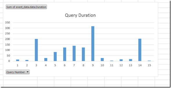
Here’s an example PivotChart showing query durations built from this data after it has been loaded to the Excel Data Model:

Not very useful, for sure, but in the next post you’ll see a more practical use for this function.

You can download the sample workbook for this post here.

The video of my SQLBits conference session “Building a reporting solution using Power Query” is now available to view (for free) on the SQLBits website:

http://sqlbits.com/Sessions/Event14/Building_A_Reporting_Solution_Using_Power_Query

It’s not your normal Power Query session about self-service ETL – instead it’s about using Power Query to create a SSRS-like reporting solution inside Excel. This is a topic I’ve been thinking about for a while, and while I have blogged about some of the tricks I show in the session (like this one about using slicers to pass parameters to Power Query) there’s a lot of new material in there too that should interest all you Power Query fans.

Of course there are literally hundreds of other great videos to watch for free at http://sqlbits.com/content/ including many others on Power BI, Power Pivot and Power Query. Alas my “Amazing Things You Can Do With Power BI” session video hasn’t been posted yet though…

[Don’t forget I’m running public Power BI and Power Query training courses in London next month! Full details at http://technitrain.com/courses.php]

There were a couple of big (well, big if you’re a Power Query fan like me) announcements made today by Miguel Llopis at the PASS BA Conference:

• Today Power Query is available only to people who have Excel Professional Plus or Excel standalone, but as of May a version of Power Query will be available on every Excel SKU. There will be some limitations around data sources that are supported if you don’t have Excel Professional Plus, but that’s ok – this change will make it much easier for people to learn about and use Power Query, and I’m really happy about that.
• Other new features coming in the May update of Power Query include the ability to turn off prompts about native database queries (useful in this scenario, for example), OData v4.0 support, the ability to use alternative Windows credentials to run queries, and a couple of new transformations such as removing empty rows.
• Excel 2016 – where Power Query is now native to Excel – will have support for creating Power Query queries using VBA and macro recording. I understand you won’t be able to edit individual steps in a query, but you’ll be able to create and delete queries programmatically and change where they load their data too.
• Excel 2016 will also support undo/redo for Power Query and give you the ability to copy/paste queries (even from workbook to workbook).
• There was a commitment that Power Query in Excel 2016 will keep getting updates on a regular basis, rather than get tied to the much slower Office release cycle, so it retains parity with the Power Query functionality in the Power BI Dashboard Designer.

All very cool stuff!

In part 1 of this series I showed how to use Power Query to extract Extended Event data generated by SSAS. Having done that, I now want to show the first (I hope of many) examples of how this data can be used for performance tuning: analysing activity in the Storage Engine, the part of SSAS that reads data from disk and aggregates it up.

I won’t go into the technical details of how I’ve used Power Query to crunch this data; you can download the sample workbook here and see for yourself. There’s nothing particularly complex going on. In brief, what I’ve done is the following:

• Called the function shown in part 1 to get the raw Extended Event data
• Filtered that data so that only the Query End, Query Subcube Verbose and Progress Report End events are left
• Calculated the start time of each event relative to the start time of the earliest recorded event, to make plotting these events on a waterfall chart possible
• Built an Excel report, including various Power Pivot measures, some normal slicers to make it easy to filter the data, some disconnected slicers for filtering so you only see events that started within a given time range, and a PivotChart showing the waterfall chart (since Excel doesn’t support this type of chart natively, I’ve used this technique to reproduce a waterfall chart with a stacked bar chart)

Here’s an example screenshot of the result, showing Storage Engine activity for a single query:

Though it’s hard to see the details at this resolution, the yellow line is the Query End event associated with the query, the grey lines are the Query Subcube Verbose events associated with the query, and the brown lines are the Progress Report events associated with each Query Subcube Verbose event.

What could this be used for? Here are some ideas:

• Looking for times when there are a lot of queries running simultaneously – and which, as a result, may be performing poorly.
• Looking for long-running Query Subcube Verbose and Progress Report End events which could be optimised by the creation of aggregations.
• Visualising the amount of parallelism inside the Storage Engine, in particular the number of Progress Report End events that are running in parallel. This would be very interesting for queries using distinct count measures when you are testing different ways of partitioning your measure group.
• Highlighting situations where calculations are being evaluated in cell-by-cell mode. When this happens you typically see a very large number of Query Subcube Verbose events being fired off within a query.

I’d like to stress once again that the object of this exercise is not to show off a ‘finished’ tool, but to show how Power Query, Power Pivot and Excel can be used for self-service analysis of this data. This workbook is just a starting point: if you wanted to use this on your own data it’s extremely likely you’d need to change the Power Query queries, the Power Pivot model and the report itself. Hopefully, though, this workbook will save you a lot of time if you do need to understand what’s going on in the Storage Engine when you run an MDX query.

Last year I blogged about how to introduce a delay between web service requests in M code. Since then a new function has been added to Power Query which makes this a lot easier: Function.InvokeAfter(). This function doesn’t seem to be documented anywhere apart from the Power Query language reference (downloadable from here); the signature is as follows:

Function.InvokeAfter(function as function, delay as duration) as any

It invokes a function after waiting for a given amount of time. Here’s a simple example of how it can be used that declares a function which returns the current date/time as text, then calls it twice with a five second delay in between:

let
    GetTimeAsText = ()=> DateTime.ToText(DateTime.LocalNow()),
    Output = GetTimeAsText() & " " 
                   & Function.InvokeAfter(GetTimeAsText, #duration(0,0,0,5))
in
    Output

The output of this query (at the time of writing) is:

28/04/2015 23:06:38 28/04/2015 23:06:43

One thing that did confuse me a bit was the fact that Function.InvokeAfter() doesn’t allow you to pass a list of arguments for the function you’re invoking like Function.Invoke(). The nice people at Microsoft helped me out with this though, and here’s a slightly more complicated example showing how to use Function.InvokeAfter() with a function that appends “Hello “ to a person’s name:

let
    SayHello = (personname as text) as text => "Hello " & personname,
    Output = Function.InvokeAfter(()=>SayHello("Chris"), #duration(0,0,0,5))
in
    Output

I saw an interesting post the other day on the Power Query Technet forum which showed how the List.Buffer() function could be used to improve calculation performance. This is something I’d seen hinted at in other places so I thought it was worth a bit of investigation.

Consider the following query:

let
    //Connect to SQL Server
    Source = Sql.Database("localhost", "adventure works dw"),
    //Get first 2000 rows from FactInternetSales
    dbo_FactInternetSales = Table.FirstN(
          Source{[Schema="dbo",Item="FactInternetSales"]}[Data], 
          2000),
    //Remove unwanted columns
    RemoveColumns = Table.SelectColumns(
          dbo_FactInternetSales,
          {"SalesOrderLineNumber", "SalesOrderNumber","SalesAmount"}),
    //Get sorted list of values from SalesAmount column
    RankValues = List.Sort(RemoveColumns[SalesAmount], Order.Descending),
    //Calculate ranks
    AddRankColumn = Table.AddColumn(RemoveColumns , "Rank", 
          each List.PositionOf(RankValues,[SalesAmount])+1)
in
    AddRankColumn

It gets the first 2000 rows from the FactInternetSales table in the Adventure Works DW database, removes most of the columns, and adds a custom column that shows the rank of the current row based on its Sales Amount.

On my laptop it takes around 35 seconds to run this query – pretty slow, in my opinion, given the amount of data in this table.

However, using the List.Buffer() function in the RankValues step like so:

let
    //Connect to SQL Server
    Source = Sql.Database("localhost", "adventure works dw"),
    //Get first 2000 rows from FactInternetSales
    dbo_FactInternetSales = Table.FirstN(
          Source{[Schema="dbo",Item="FactInternetSales"]}[Data], 
          2000),
    //Remove unwanted columns
    RemoveColumns = Table.SelectColumns(
          dbo_FactInternetSales,
          {"SalesOrderLineNumber", "SalesOrderNumber","SalesAmount"}),
    //Get sorted list of values from SalesAmount column
    //And buffer them!
    RankValues = List.Buffer(List.Sort(RemoveColumns[SalesAmount], Order.Descending)),
    //Calculate ranks
    AddRankColumn = Table.AddColumn(RemoveColumns , "Rank", 
          each List.PositionOf(RankValues,[SalesAmount])+1)
in
    AddRankColumn

Makes the query run in just 2 seconds. The List.Buffer() function stores the sorted list of values used to calculate the rank in memory which means it will only be evaluated once; in the original query it seems as though this step and those before it are being evaluated multiple times. Curt Hagenlocher’s comment (on this thread) on what List.Buffer() does for a similar calculation is telling:

The reason for this is that M is both functional and lazy, so unless we buffer the output of List.Select, we’re really just building a query that needs to be evaluated over and over. This is similar to the Enumerable functions in LINQ, if you’re familiar with those.

Table.Buffer() and Binary.Buffer() functions also exist, and do similar things.

A few other points to make:

• This is not necessarily the optimal way to calculate ranks in Power Query – it’s just an example of how List.Buffer() can be used.
• In the first query above, query folding is not taking place. If it had been it’s likely that performance would have been better. Since using List.Buffer() explicitly prevents query folding from taking place, it could make performance worse rather than better because of this in many cases.
• I’m 100% certain you’ll get much better performance for a rank calculation by loading the table to the Excel Data Model/Power Pivot and writing the calculation in DAX. You should only really do calculations like this in Power Query if they are needed for other transformations in your query.

Quite often, in Power Query, you want to ‘nest’ calculations and transformations – apply them not across the whole table, but repeat the same calculation or transformation across multiple groups of rows within that table. Let me give you an example…

Take the following input table:

Imagine you wanted to add a column showing the rank of each row by Sales. In Power Query you would just need to:

1. Load the data
2. Sort the table in descending order by Sales
3. Add an index column starting at 1, which is the rank

You would end up with the following output:

…and here’s the M code, all of which is generated by the UI:

let
    Source = Excel.CurrentWorkbook(){[Name="Sales"]}[Content],
    #"Sorted Rows" = Table.Sort(Source,{{"Sales", Order.Descending}}),
    #"Added Index" = Table.AddIndexColumn(#"Sorted Rows", "Rank", 1, 1)
in
    #"Added Index"

Now imagine you wanted to rank Sales within each month. That’s to say you want to apply the same steps as shown in the previous query but for each month individually to get an output like this:

One way to tackle this, and problems like it, is to do the following. First, do a Group By on the column you want to repeat the calculation over, in this case Month, and use the All Rows aggregation operation. This will result in a table with one row for each month and a column containing nested tables, as shown below:

Each one of these tables contains the rows from the original table for the month.

You can then take your original transformation and turn it into a function, either in a separate query or as a step in your current query. Here’s an example of how the query above can be turned into a function that takes a table and returns a table with a rank column added:

(tabletorank as table) as table =>
     let
      SortRows = Table.Sort(tabletorank,{{"Sales", Order.Descending}}),
      AddIndex = Table.AddIndexColumn(SortRows, "Rank", 1, 1)
     in
      AddIndex

Next, you need to pass each nested table to this function. You could do that in a calculated column, but the most elegant way I think is by using the Table.TransformColumns() function which takes a function and applies it to every value in a column (see here for another example of how to use it).

Finally, you get the final output by clicking on the Expand icon in the AllRows column and then choosing to expand all the columns in the nested table except the ones you originally grouped on:

Here’s the full M code:

let
    //Get data from Excel
    Source = Excel.CurrentWorkbook(){[Name="Sales"]}[Content],
    //Group by Month
    Grouped = Table.Group(Source, {"Month"}, {{"AllRows", each _, type table}}),
    //Declare a function that adds a Rank column to a table
    RankFunction = (tabletorank as table) as table =>
     let
      SortRows = Table.Sort(tabletorank,{{"Sales", Order.Descending}}),
      AddIndex = Table.AddIndexColumn(SortRows, "Rank", 1, 1)
     in
      AddIndex,
    //Apply that function to the AllRows column
    AddedRank = Table.TransformColumns(Grouped, {"AllRows", each RankFunction(_)}),
    //Expand the tables in the AllRows column again
    ExpandAgain = Table.ExpandTableColumn(AddedRank, "AllRows", 
       {"Product", "Sales", "Rank"}, {"Product", "Sales", "Rank"})
in
    ExpandAgain

You can download the example workbook here.

This pattern could also be applied to other types of calculation that need to be nested, for example running totals or shares.

One problem that can really drive you crazy when working with data from text files is the many different formats that dates and numbers can be stored in around the world. For example, take a look at the contents of a tab-delimited file shown in the following screenshot:

There’s a single row of data and two columns, Date and Sales. What number and date are shown though? For me, living in the UK, the date shown is the 2nd of March 2015 (in the UK, like most of the world, we use the DD/MM/YYYY date format) and the number is one hundred thousand and two (in the UK we use the . sign as a decimal separator and the , as a thousands separator). However, if I was from the US and used the MM/DD/YYYY format I’d read the date as the 3rd of February 2015; and if I was from France and used a comma as a decimal separator, I’d read the number as a value just a tiny amount over one hundred. Of course, if you’re working in one country and getting data sent from another, which uses a different date or number format, you need to take all of these variations into account.

The good news is that Power Query has a really easy way of doing this for you, even if it’s not immediately obvious where this functionality is. You don’t need to change your Windows locale or split dates into their constituent parts and rearrange them in the correct order, or anything like that.

When you first load a csv file like the one shown above into Power Query, it will try to guess the data types of each column. Here’s the code generated by Power Query for this file:

let
    Source = Csv.Document(
                       File.Contents(
                        "C:\Users\Chris\Documents\Power Query demos\PQDateNumberFormats.csv"),
                        null,"#(tab)",null,1252),
    #"First Row as Header" = Table.PromoteHeaders(Source),
    #"Changed Type" = Table.TransformColumnTypes(
                                     #"First Row as Header",
                                     {{"Date", type date}, {"Sales", Int64.Type}})
in
    #"Changed Type"

As you can see, it has created three steps in the query automatically:

1. Source loads the data from the CSV file given and sees that it’s tab delimited
2. First Row as Header uses the first row of data as the column headers
3. Changed Type sets the Date column to be type date, and Sales to be an integer

To change how the column data types are interpreted though, you first need to delete the Changed Type step by clicking on the cross icon next to it, shown above. Then, right-click on the Date column, choose Change Type then Using Locale…

When you do this, the Change Type With Locale dialog appears:

A locale is simply a name for all of the rules for date and number formats and more associated with a particular language and region. So, for example, setting the Date column so that it is interpreted using the English (United States) locale, means that when the data is loaded into Power Query on my machine I see the date 3/2/2015.

What’s happened is that the csv file contains the date “2/3/2015”, I have told Power Query that the data source uses a US English format date, Power Query has then assumed this date is therefore in MM/DD/YYYY format, loaded the data for me and shown the date in my own locale (which is English (United Kingdom)) in DD/MM/YYYY format as 3/2/2015. The date itself hasn’t changed, just the way it is displayed.

Using the same technique to import the Sales column as a decimal value using the English United States locale like so:

…gives the following final result, where the comma is assumed to be a thousands separator:

Here’s the new code for the query:

let
    Source = Csv.Document(
                      File.Contents(
                       "C:\Users\Chris\Documents\Power Query demos\PQDateNumberFormats.csv"),
                       null,"#(tab)",null,1252),
    #"First Row as Header" = Table.PromoteHeaders(Source),
    #"Changed Type with Locale" = Table.TransformColumnTypes(
                        #"First Row as Header", 
                        {{"Date", type date}}, "en-US"),
    #"Changed Type with Locale1" = Table.TransformColumnTypes(
                        #"Changed Type with Locale", 
                        {{"Sales", type number}}, "en-US")
in
    #"Changed Type with Locale1"

However, if I change the locale used to set the types of these two columns to French (France), I see the following:

You will see that I have told Power Query to interpret the value “100,002” as a decimal number using a French format, where a comma is used as a decimal separator, and it has therefore imported and displayed it as 100.002 in the English (United Kingdom) format with a decimal point used as the decimal separator.

Recently, I was working with a customer that wanted to be able to draw lines between two points in Power Map. At the time I thought the only way that it might be possible was by using Power Query to generate a table of data containing a series of points that were so close together that they looked like a single line, and then plot these points in Power Map (similar to what I show in the screenshot here). Soon after, the new custom regions functionality was released in Power Map (there’s no documentation I can find right now, but this blog post is reasonably detailed) and I wondered whether now it might be possible to draw lines. Unfortunately not: Power Map can now import SHP and KML files, but it doesn’t support all the features of KML – only polygons (and even then not all the features of polygons, although inner and outer boundaries work fine). I guess this is ok for the primary use-case of Power Map, which is plotting BI data on a map, but it would be nice to see more KML features supported so that Power Map can show richer supporting information for the data: things like arrows showing direction of travel, and so on.

Anyway, I then thought – why not use polygons to draw these lines? Again, I hit a slight problem: I wanted to generate the polygons for the lines in code, and Power Map can only import SHP or KML data from files. It would be really useful if we could use shape data stored in the Excel Data Model… but we can’t. However, it is possible to use Power Query to generate KML and then copy and paste this code into a file, which can then be imported into Power Map. So, just for the fun of it, I put together a proof-of-concept workbook containing Power Query queries to generate all the tables and KML code needed to draw lines between two places, and a Power Map tour that shows the output. Here’s what the end result looks like:

You can download my example workbook that contains all the code, plus all the supporting files, here. You will need to update some file paths in the M code to get it all to work.

The starting point is two tables on the worksheet, one containing the single starting point for the lines, the other all of the destinations:

There’s a lot of M code so I’m not going to include it in this post, but here’s an overview of what each query does:

• GetLatLong is a function that calls the Bing Maps REST API to find the latitude and longitude for each place in the tables above. You will need your own Bing Maps account key if you want to use this code yourself – you can get one at https://www.bingmapsportal.com/
• Starting Point and Ending Points simply load the data from the Excel tables
• StartingPointLatLong gets the latitude and longitude of the starting point by calling GetLatLong
• StartEndPoints gets the latitude and longitude of all the ending points by calling GetLatLong, adds custom columns to show the starting point name, latitude and longitude against each ending point, and loads the result to the Excel Data Model. You have to have some data in the Excel Data Model for Power Map to display the lines, and it’s important that Power Map can match the values in one column in this table with the names of objects in the KML file.
• BasicPolygonTemplate loads a fragment of KML, containing the definition of a polygon, from a text file. This contains two ‘parameters’, @Name and @Coordinates, which will be overwritten using Text.Replace() later on when the actual KML is being generated.
• GetCoordinateList is a function to draw a rectangular polygon that represents the line between the starting point and an ending point. I had a lot of fun trying to get the code for this working properly (I wish I could remember any of the trigonometry that I learned after the age of 13…) and I’m still not convinced the rectangles are properly rectangular, but they’re good enough.
• KML generates the KML for all of the polygons. The output of this query must be copied from the Power Query query window into a text file with the .kml extension, for example Test.kml. There’s no need to load the output of this query to anywhere.

With all of that done, you now need to open Power Map and create a new tour. Choose EndingPoint as the sole Geography column, then choose Custom Region (.kml, .shp) from the dropdown list below and click Yes to import custom regions.

Select the .kml file you created earlier, containing the output of the KML Power Query query, and then click Import:

Finally, change the visualisation type to Region and optionally add Ending Point to Category to make the lines different colours:

And bingo, you see the lines:

Support for custom regions is a massive step forward for Power Map in my opinion: rather than just being a toy for creating flashy demos it’s now able to handle a lot more real-world requirements. However, having some way of programmatically creating regions and shapes (either through Power Query as I’ve done here, or using VBA or some other API), being able to load shape data from the Excel Data Model, or even just to be able to draw shapes on a map manually, would be welcome. I’m no mapping expert but I’ve come across a few frustrated Mappoint (which was discontinued at the end of 2014) users who would like to use Power Map but find that it can’t do everything that they need. The code in this post shows what’s possible but it’s still way too complex for most users and hardly an elegant solution.

In Excel 2016, Power Query is no longer an Excel add-in but a native feature of Excel, and what’s more, you can now use VBA to create and manage Power Query queries.

I’ve found two sources of information about how to use VBA with Power Query in Excel 2016. First, there are some code samples on the Technet Gallery here:
https://gallery.technet.microsoft.com/VBA-to-automate-Power-956a52d1#content
…and Gil Raviv, a Program Manager at Microsoft, has also asked for feedback on this functionality on this thread:
https://social.technet.microsoft.com/Forums/en-US/1eac9c36-b6e4-48f0-a51a-fa92b24cf1d9/vba-and-power-query-in-excel-2016-preview-lets-get-started?forum=powerquery

Secondly, I was contacted recently by Tycho Grouwstra who shared with me some of the interesting work he has done using VBA and Power Query in the Excel 2016 Preview, and who has very kindly allowed me to blog about it here. His work is much more representative of how I think most people will want to use this feature.

Tycho sent me a .xlsm file containing all of the VBA code, which you can download here. Obviously the code only works in the Excel 2016 Preview, but you can still open the file and look at the code in Excel 2013. However if you’re worried about downloading a workbook with macros in, I extracted the code to a text document which you can see here. If you want to copy the code to use in your own workbook, you’ll need to go to the VBA Editor, select Tools/References and add a reference to “Microsoft ActiveX Data Objects 6.1 Library”.

The VBA code includes examples of how to:

• Delete all the Power Query queries in a workbook
• Export/import the M code for all queries to/from another Excel workbook
• Export/import the M code for all queries to text files
• Refresh all the Power Query queries in the workbook
• Load a query to an Excel table

A few bugs/features in the Preview are also pointed out, namely:

• Imported queries don’t always show up in the Workbook Queries pane; the workaround is to close and reopen the workbook
• Functions aren’t recognised as functions (ie they don’t have the fx icon) until you open the Query Editor and the Close & Load
• Query groups aren’t supported yet – which is a bit of an oversight, in my opinion, but the forums thread linked to above indicates it won’t be addressed before RTM unfortunately
• Loading the output of a query into an Excel table using the code given here doesn’t seem to have the same result as loading a query to a table in the worksheet using the Power Query UI: it creates a blue, rather than green, table that doesn’t always retain row order.

I can imagine a lot of serious Power Query users will create workbooks containing a library of their most useful queries and functions, and use VBA code to copy these queries and functions into new workbooks as and when necessary. We’ll have to wait and see what Microsoft’s plans for sharing Power Query queries are, whether they’ll go beyond what’s already been seen in Office 365 Power BI, whether they will be part of a bigger bundle of services and what the cost will be.

Incidentally, the sample workbook contains a lot of interesting, generally useful Power Query queries and functions written by Tycho and others which is also available in the following GitHub repository: https://github.com/tycho01/pquery

Disappearing or renamed columns in your data source can cause all kinds of problems when you’re importing data using Power Query: errors when you try to refresh the query, broken calculations in Power Pivot, PivotTables that reformat themselves and then need to be manually recreated. As a result, it can be a very good idea to build some logic into your Power Query queries that ensures that a table always contains the columns you’re expecting.

Consider the following csv file:

In Power Query, if you connect to it and create a query you’ll end up with something like this:

let
    Source = Csv.Document(File.Contents("C:\Demo.csv"),null,",",null,1252),
    #"First Row as Header" = Table.PromoteHeaders(Source),
    #"Changed Type" = Table.TransformColumnTypes(#"First Row as Header",{{"Sales", Int64.Type}})
in
    #"Changed Type"

Let’s assume that this query is called GetSourceData. Let’s also assume that your output from Power Query should always be a table that has the three columns Product, Month and Sales, and that Product and Month should be text columns and Sales should be numeric. The basic steps to take to ensure that this always happens, even if the columns in the csv file change, are as follows:

1. Create a query that connects to your data source, for example like GetSourceData above
2. Create a query that will always return a table with the columns you want, but which contains no rows
3. Append the second table onto the end of the first table. This will result in a table that contains all of the columns from both tables.
4. Remove any unwanted columns.

There are a number of ways to create the empty table needed in step 2. You could use the #table() function if you’re confident writing M code, and the following single line query (no Let needed) does the job:

#table(
 type table [Product=text, Month=text, Sales=number],
 {})

Alternatively, if you wanted something that an end user could configure themselves, you could start with a table in Excel like this:

then transpose it, use the first row of the resulting table as the header row, then set the data types on each table to get the same output:

let
    Source = Excel.CurrentWorkbook(){[Name="Columns"]}[Content],
    #"Transposed Table" = Table.Transpose(Source),
    #"First Row as Header" = Table.PromoteHeaders(#"Transposed Table"),
    #"Changed Type" = Table.TransformColumnTypes(#"First Row as Header",
	{{"Product", type text}, {"Month", type text}, {"Sales", Int64.Type}})
in
    #"Changed Type"

Assuming that this query is called ExpectedColumns, it’s then a trivial task to create a third query that appends the ExpectedColumns query onto the end of the GetSourceData query. If GetSourceData includes all the columns it should then this append will have no effect at all; if some of the columns have changed names or disappeared, you’ll see all of the columns present from both GetSourceData and ExpectedColumns in the output of the append. For example if the Month column in GetSourceData is renamed Months then the output of the append will look like this:

Finally, in this third query you need to select all the columns you want (ie all those in the ExpectedColumns query) and right click/Remove Other Columns, so you remove all the columns you don’t want. In the previous example that gives you:

The point here is that even though the Month column only contains nulls, and the actual month names have been lost, the fact that the columns are all correct means that you won’t get any errors downstream and your PivotTables won’t be reformatted etc. Once you’ve fixed the problem in the source data and refreshed your queries, everything will go back to normal.

Here’s the code for this third query:

let
    Source = GetSourceData,
    Append = Table.Combine({Source,ExpectedColumns}),
    #"Removed Other Columns" = Table.SelectColumns(Append,{"Product", "Month", "Sales"})
in
    #"Removed Other Columns"

For bonus points, here’s another query that compares the columns in GetSourceData and ExpectedColumns and lists any columns that have been added to or are missing from GetSourceData:

let
    //Connect to Excel table containing expected column names
    ExcelSource = Excel.CurrentWorkbook(){[Name="Columns"]}[Content],
    //Get list of expected columns
    ExpectedColumns = Table.Column(ExcelSource, "ColumnName"),
    //Get a list of column names in csv
    CSVColumns = Table.ColumnNames(GetSourceData),
    //Find missing columns
    MissingColumns = List.Difference(ExpectedColumns, CSVColumns),
    //Find added columns
    AddedColumns = List.Difference(CSVColumns, ExpectedColumns),
    //Report what has changed
    OutputMissing = if List.Count(MissingColumns)=0 then
                     "No columns missing" else
                     "Missing columns: " & Text.Combine(MissingColumns, ","),
    OutputAdded = if List.Count(AddedColumns)=0 then
                     "No columns added" else
                     "Added columns: " & Text.Combine(AddedColumns, ","),
    Output = OutputMissing & "   " & OutputAdded
in
    Output

You can download the sample workbook for this post here.

Something I was meaning to mention in my previous post (but forgot about…) was that in a lot of cases you don’t really care if your output contains all the required columns – it’s enough just to check that your input contains all the required columns. Luckily M has a function called Table.HasColumns() to help you do this. For example, using the csv source file from my previous post, which should have three columns called Product, Month and Sales, the following query will return true if the source file has these columns and false if it doesn’t:

let
    Source = Csv.Document(File.Contents("C:\MissingColumnDemo.csv"),[Delimiter=",",Encoding=1252]),
    PromotedHeaders = Table.PromoteHeaders(Source),
    CheckColumns = Table.HasColumns(PromotedHeaders, {"Product", "Month", "Sales"})
in
    CheckColumns

Every time there’s a new release of Power Query or Power BI Desktop, I always check to see if there are any interesting new M functions that have been added (I used #shared to do this, as detailed here). For the RTM version of Power BI Desktop I spotted two new functions:

As well as ODBC connections, we can now use OLEDB and ADO.NET data sources – although they aren’t shown in the UI yet. And you know what this means… with an OLEDB connection we can now run our own MDX and DAX queries against SSAS data sources! I assume this will be coming in Power Query in Excel soon too.

Here’s an example query showing how to use OleDB.Query() to run an MDX query against the Adventure Works DW cube in SSAS Multidimesional:

let
    Source = OleDb.Query(
              "Provider=MSOLAP.5;Data Source=localhost;
               Initial Catalog=Adventure Works DW 2008", 
              "select {measures.[internet sales amount]} on 0, 
               [date].[calendar].[calendar year].members on 1 
               from [adventure works]"
             )
in
    Source

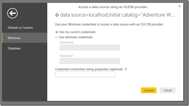
As you can see, it’s pretty straightforward: you just need to supply a connection string and a query. You will need to tell Power BI Desktop which credentials to use when running the query the first time you connect to SSAS, and that’s probably going to be Windows:

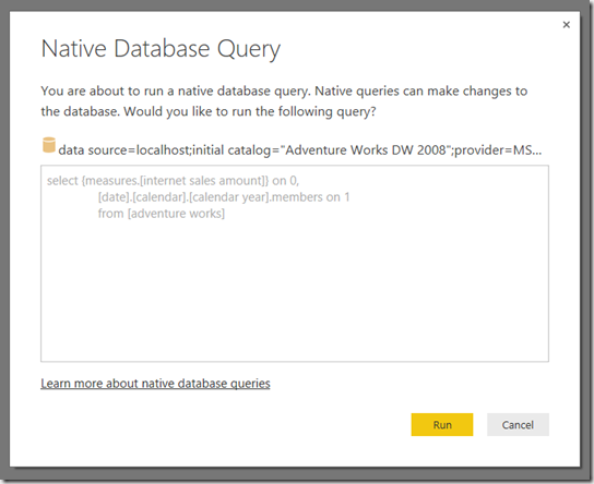
You will also see a prompt the first time you run the query, asking for permission to run a Native Database Query:

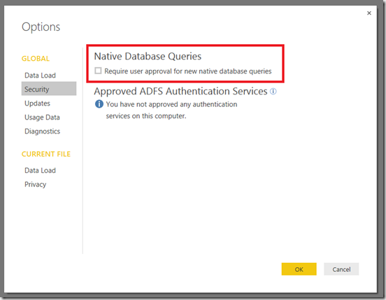
This prompt will appear each time a different MDX query is run; you can turn off this prompt in the Options dialog on the Security tab by unchecking the Require user approval for new native database queries box:

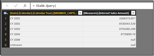
Here’s the output of the MDX query from the example code: