Quantcast
Channel: Chris Webb's BI Blog: Power Query
Viewing all 252 articles
Browse latest View live

Returning Error Messages As Well As Results In Power Query

$
0
0

Back in September I wrote a post on handling situations where the data source for your Power Query query was unavailable. The great thing about that technique is that instead of seeing an error message when you refresh your query, instead you get an empty table with the same structure – which means that the Excel Data Model doesn’t get messed up, you don’t lose relationships and all your PivotTables remain intact. However it means you no longer see the error message (unless you return it in the table somehow, which isn’t ideal), which makes it hard to debug. What you really want is to get the empty table AND the error message somehow. But surely a Power Query query can only return a single value as an output?

Actually no. Every value in M can have a metadata record associated with it, and we can use this here to our advantage (I’ve been wondering whether there was a use for metadata ever since I read about it in the Language spec… and at long last I’ve found one!). Here’s a simple example of a query that shows how to associate a metadata record with a value:

let
    Source = "Some Random Value" meta [message = "Hello World", somenumber = 123],
    Output = Source
in
    Output


The output of this query is just the text “Some Random Value”:

image

At this point we’re setting the metadata but not doing anything with it. The following query uses the Value.Metadata() function to get the metadata record:

let
    Source = "Some Random Value" meta [message = "Hello World", somenumber = 123],
    Output = Value.Metadata(Source)
in
    Output


The output is now a record value:

image 

Basically, this means that in scenarios where we want to handle a data source error we can always return a table and at the same time return any error messages in the metadata.

Here’s a similar scenario to the one I showed in my original blog post, but where the query does a select distinct on the EnglishDayNameOfWeek column in the DimDate table in the Adventure Works DW database:

let
    //Connect to SQL Server
    Source = Sql.Database("localhost", "adventure works dw"),
    //Get DimDate table
    dbo_DimDate = Source{[Schema="dbo",Item="DimDate"]}[Data],
    //Remove all other columns except EnglishDayNameOfWeek
    #"Removed Other Columns" = Table.SelectColumns(dbo_DimDate,{"EnglishDayNameOfWeek"}),
    //Get distinct values from this column
    #"Removed Duplicates" = Table.Distinct(#"Removed Other Columns"),
    //Output in case of error
    AlternativeOutput=#table(type table [EnglishDayNameOfWeek=text], {}),
    //Does the Removed Duplicates set error?
    TestForError= try #"Removed Duplicates",
    Output = if TestForError[HasError]
             then
             //In case of error return empty table
             //and attach error message in metadata
             (AlternativeOutput meta [message = TestForError[Error]])
             else
             //If there's no error
             //just return the table plus a message
             (#"Removed Duplicates" meta [message = "Query executed successfully"])
in
    Output


The output when the query (called DimDate) executes successfully, shown in an Excel table, is just a list of day names:

image

You can now create a second query in the same workbook with the following definition to get the metadata record associated with the output of this query:

let
    Source = Value.Metadata(DimDate),
    message = Source[message]
in
    message

The output of this query, when the first query is successful, is:

image

However, if you rename the EnglishDayNameOfWeek column in SQL Server, the first query now returns an empty table:

image

The second query now returns the error message when it’s refreshed:

image

One thing to be careful of, bearing in mind what we learned about Power Query and M in my last post, is that the output of the first query is not cached after it has been executed so executing the second query to get the error message will involve at least a partial re-execution of the first query. However in this particular case if you look in Profiler you can see Power Query checking to see whether the EnglishDayNameOfWeek column exists in the DimDate table before it tries to do the select distinct SQL query, and this is enough to know whether the query will fail or not – so whether there is an error or not, running the second query to get the message does not result in the (potentially expensive) select distinct SQL query being executed.

You can download the sample workbook for this post here.


Combining Data From Multiple Excel Workbooks With Power Query–The Easy Way!

$
0
0

If there’s one feature of Power Query that’s guaranteed to get Excel users very, very excited indeed it’s the ability to combine data from multiple workbooks into a single table. The bad news is that this is something that Power Query can’t do through the user interface (although so many people have asked for it I wouldn’t be surprised if it gets added to the product soon) and it’s not obvious how to do it.

This is a topic that has been blogged about many times over the past year or so (see DutchDataDude, Mike Alexander, Ken Puls, Miguel Escobar – apologies to anyone I’ve missed) so why should I write about it? Well, all these other posts show you the steps you have to go through to build your own function and then use that function inside a query, which is fine, but it involves a lot of clicking and typing code each time you want to do it. It’s all very time-consuming if you don’t know Power Query that well, though, and not something a regular Excel user would want to do. I’ve got an easier way though: a generic function that can combine data from workbooks in any folder you point it at. Once you’ve created it it’s very easy for anyone to use, can be reused over and over, and of course you can share this function through the Power BI Data Catalog if you have a Power BI for Office 365 subscription.

Steps to add the Power Query function to your workbook

You can either follow the steps below to add the function to your workbook, or instead just download the sample workbook containing the function here – which is a lot quicker!

1) Copy the following code onto the clipboard

//Define function parameters
(#"Directory containing Excel files to combine" as text,
optional #"Name of each Excel object to combine" as text,
optional #"Use first rows as headers" as logical) =>
let
    //If the optional Excel object name parameter is not set, then default to Sheet1
    ExcelName = if #"Name of each Excel object to combine" = null
                then "Sheet1"
                else #"Name of each Excel object to combine",
    //If the optional Use first rows as headers parameter is not set, then default to true
    UseFirstRowsAsHeaders = if #"Use first rows as headers"= null
                            then true
                            else #"Use first rows as headers",
    //Get a list of all the files in the folder specified
    Source = Folder.Files(#"Directory containing Excel files to combine"),
    //Filter these to only get Excel files
    OnlyGetExcelFiles = Table.SelectRows(Source,
                              each ([Extension] = ".xlsx")
                              or ([Extension] = ".xls")),
    //Find the full path of each file
    FullPath = Table.CombineColumns(
                    OnlyGetExcelFiles ,
                    {"Folder Path", "Name"},
                    Combiner.CombineTextByDelimiter("", QuoteStyle.None),"Merged"),
    //Get a list containing each file path
    ExcelFiles = Table.Column(FullPath, "Merged"),
    //Define a function to get the data from the specified name in each Excel workbook
    GetExcelContents = (FileName as text) =>
     let
      //Connect to the workbook
      Source = Excel.Workbook(File.Contents(FileName), UseFirstRowsAsHeaders),
      //Get a table of data from the name specified
      //If the name doesn't exist catch the error and return null
      ExcelData = try Source{[Item=ExcelName]}[Data]
                           otherwise try Source{[Name=ExcelName]}[Data]
                           otherwise null
     in
      ExcelData,
    //Call the above function for each Excel file
    ReadAllWorkbooks = List.Transform(ExcelFiles, each GetExcelContents(_)),
    //Remove any null values resulting from errors
    IgnoreNulls = List.RemoveNulls(ReadAllWorkbooks),
    //Combine the data from each workbook into a single table
    CombineData = Table.Combine(IgnoreNulls)
in
   CombineData


2) Open Excel and go to the Power Query tab on the ribbon. Click on the From Other Sources button and then click Blank Query.

image

3) The Power Query query editor window will open. Go to the View tab and click on the Advanced Editor button.

image

4) The Advanced Editor will open. Delete all the code in the main textbox and replace it with the code above. Click OK to close the Advanced Editor.

image

5) In the Query Settings pane on the right-hand side of the Query Editor, change the name of the query to CombineExcel, then go to the Home tab on the ribbon and click the Close & Load button. The Query Editor will close.

image

image

6) You can now see your function in the Workbook Queries pane in Excel! It should look like this:

image


Using the function to combine data from multiple workbooks

To use the function, double-click on it in the Workbook Queries pane or right-click and select Invoke. The following dialog will appear:

image

You can enter three parameters here:

  • The path of the directory containing the Excel workbooks that you want to read data from. The function can read from xlsx and xls files (though for the latter to work you need the Access 2010 engine installed, a free download if you only have Excel 2013) and will ignore any other files in the folder. The function will also read any Excel files in any subfolders.
  • Where you want to get data from in each Excel workbook. This can be the name of a worksheet (for example you could enter Sheet2 here) or a named range or a table. It’s an optional parameter so if you leave it blank it will get data from the worksheet Sheet1. If a workbook doesn’t contain the name you enter here it will be ignored. If the format of the data in each worksheet is not consistent (for example if you have different column names) then be warned: you may get some strange results.
  • Whether data on your worksheet (if you’re getting data from a worksheet) contains headers. Enter true here if your data does have a header row in every worksheet; false otherwise. This is also an optional parameter and if you leave this box empty the default value is true.

When you click OK, a new Power Query query will be created, the Query Editor window will open and you’ll see all the data from all of the Excel workbooks combined. The first step of this query is a call to the CombineExcel() function and you can carry on working with your data in Power Query as normal.

image

Disclaimer: I’ve done a reasonable amount of testing on this and I’m pretty sure it works well, but of course there will be bugs. Please leave a comment if you find a bug or can suggest any other improvements.


Power Query Now Works With SSAS

$
0
0

I normally don’t bother blogging when one of the Power Query monthly updates gets released – the posts on the Power BI blog have all the details and there’s nothing more to add. This month’s update, though, sees Power Query able to use SSAS Multidimensional and Tabular models as a data source (you can read the announcement here and watch the video here) and I thought that since these are my two favourite Microsoft products I should comment.

In no particular order, some observations/thoughts:

  • Power Query is generating MDX queries in the background here. And yes, query folding is taking place here so where possible the filtering and sorting is being translated back to MDX so the work is taking place on the server. I’ve had a look at the MDX being generated and while it’s a bit strange in places it’s basically good and should perform well.
  • In order to get Power Query to work I had to install the 2012 version of ADOMD, even though I already had the 2014 version installed. Hmmm.
  • It also doesn’t display calculated measures that aren’t associated with a measure group, although this is going to be fixed in a later release. In fact I experienced several errors associated with calculated measures when I first installed the new release, but these went away after I cleared the Power Query cache and rebooted.
  • This update does not support custom MDX queries, unlike the equivalent SQL Server data source; again this is on the roadmap though. This will be useful for two reasons:
    • For complex queries, or queries that have to be written in a certain way to perform well, sometimes you have to have complete control of the query
    • It would allow you to run DAX, DMX and SQL queries on SSAS, and also let you query SSAS DMVs. Custom DAX queries can perform a lot better than the equivalent MDX in some cases, and querying DMVs would allow you to build SSAS monitoring dashboards in Excel.
  • The Excel Data Model (which lots of people call Power Pivot, but I’m going to stick to my guns on this one because the Excel Data Model is not the same thing as Power Pivot) is not supported as a data source yet either, even though it can be queried in MDX just like SSAS. This would also be useful to have although I can also see it’s harder to implement, given that the Excel Data Model is both a data source and a data destination.
  • There are a whole bunch of new (well, not really new because they have been around since the support for SAP Business Objects came out this summer) M functions to generate those MDX queries. They probably deserve their own blog post at some point in the future.
  • Apart from the obvious reason that it allows you to combine data from SSAS with other data sources and/or load it into the Excel Data Model, why is it useful to have Power Query to connect to SSAS? What does it give you over and above the existing PivotTable, Excel Cube Function and Query Table connectivity? Why do we even need to extract data from a cube in the first place? 
    • This may only be a minor reason, but a lot of people still do get caught by the problem of having multiple cubes where they should have one, and need to build reports that incorporate data from multiple cubes. Power Query gives them an easy way of doing this.
    • I believe the step-based approach of Power Query makes it much easier for users to build complex queries than other SSAS front-ends, such as PivotTables. Being able to see the effect of filters and other transformations as they are applied, and being able to delete them and rearrange the order that they are applied in, is a huge benefit. Think of Power Query as being a custom MDX query builder where the output is a regular table in Excel rather than a PivotTable.
    • This last point leads me on to a topic that I’ve been thinking about a lot recently, and which will be the subject of a whole series of blog posts soon, namely that it is wrong to think of Power Query as simply a self-service ETL tool. It is that, but I also think that has a lot of potential as a self-service reporting tool too. For both relational database and SSAS I think Power Query could be very useful as a means of creating SSRS-like detail-level reporting solutions inside Excel. Problems with the MDX generated by PivotTables mean that queries with large numbers of hierarchies crossjoined together perform badly; the MDX that Power Query generates does not suffer from this problem. Functions can be used to parameterise Power Query queries (in fact earlier this evening I learned something immensely cool about function parameters that I’ll blog about later this week and which will make functions even more useful!) and can therefore be used in almost exactly the same way as datasets in SSRS.

Specifying Allowed Values, Sample Values and Descriptions For Function Parameters In Power Query–Part 1

$
0
0

The other day when I was thinking about Power Query functions (as you do) it occurred to me that they would be a lot more usable if, when you invoked them, you could show your users a dropdown box for each parameter where they could choose all of the allowed parameter values rather than expect them to type a value which may or may not be correct. I thought this was such a good idea that I sent an email to the Power Query team, and within a few hours I got a reply from Matt Masson… saying that they had already implemented this some time ago but hadn’t documented it yet. He also, very kindly sent me a code example, and allowed me to blog about it (thanks Matt!). In this post I’m going to look at a very simple example of how to do this; in part 2 I’ll show some a complex scenario involving SQL Server.

Consider the following Power Query function that multiplies two numbers:

(FirstNumber as number, SecondNumber as number) as number =>
FirstNumber * SecondNumber


Enter this into a new blank query and you’ll see the following in the Query Editor:

image

Clicking either the Invoke Function or Invoke button will make the Enter Parameters dialog appear:

image

You can then enter two numbers, click OK, and the query will invoke the function with those two numbers and show the result:

image

Now it turns out that there are three properties you can set on a function parameter to control how it is displayed in the Enter Parameters dialog:

  • A text description of the parameter
  • A sample value
  • A list of allowed values that can be passed to the parameter, that can be selected from a dropdown box

Unfortunately the way to set these properties isn’t exactly straightforward, but the basic process is this:

  • For each parameter create a custom type, and then use a metadata record to assign the property values for that type
  • Then create a custom function type, where each parameter uses the custom types created in the previous bullet
  • Finally take your existing function and cast it to your new function type using the Value.ReplaceType() function.

OK, I know, this sounds scary – and it is, a bit. Here’s how the original function can be rewritten:

let
    //declare a function
    MultiplyTwoNumbersBasic =
                             (FirstNumber as number, SecondNumber as number)
                             as number =>
                             FirstNumber * SecondNumber,
    //declare custom number types with metadata for parameters
    MyFirstNumberParamType = type number
                        meta
                        [Documentation.Description = "Please enter any number",
                         Documentation.SampleValues = {8}],

    MySecondNumberParamType = type number
                        meta
                        [Documentation.Description = "Please choose a number",
                         Documentation.AllowedValues = {1..5}],
    //declare custom function type using custom number types
    MyFunctionType = type function(
                                           FirstNumber as MyFirstNumberParamType,
                                           SecondNumber as MySecondNumberParamType)
                                    as number,
    //cast original function to be of new custom function type
    MultiplyTwoNumbersV2 = Value.ReplaceType(
                                                   MultiplyTwoNumbersBasic,
                                                   MyFunctionType)
in
    MultiplyTwoNumbersV2


Now, when you invoke the function, the Enter Parameters dialog looks like this:

image

Note how for the FirstNumber parameter the description and the sample value is displayed; and how for the SecondNumber parameter the dropdown list shows all of the allowed values in the list we declared (remember that {1..5} returns the list {1,2,3,4,5} in M) and how it is no longer possible to type a value here.

Three things to mention last of all:

  • Although Documentation.SampleValues is a list, only the first value in the list seems to be displayed
  • Documentation.AllowedValues doesn’t actually prevent you from calling the function with a value not in this list, it just controls what values are seen in the dropdown list
  • The Workbook Queries pane no longer recognises your function as a function when you do all this – it doesn’t have the special function icon, and there is no Invoke option on the right-click menu. This is a real shame because, while it doesn’t affect how the function works, it does make it much less intuitive to use and the whole point of this exercise is usability. Hopefully this gets fixed in a future build.

You can download the a sample workbook containing all the code in this post here.


New Power Query Videos Live

$
0
0

I have recorded two new videos for Project Botticelli about Power Query that are now available to view. They are:

What Is Power Query?

This is short introduction to Power Query is free to view (registration required) and covers just the basics.

https://projectbotticelli.com/knowledge/what-is-power-query-video-tutorial?pk_campaign=tt2014cwb

clip_image001


Power Query Fundamentals

This 45 minute video goes into more detail about all of the cool things you can do in the Power Query Query Editor. You’re going to need a subscription to see this, but if you subscribe you will of course get access to loads of other videos too (including my MDX course, Marco and Alberto’s DAX videos, and lots of other cool MS BI content).

https://projectbotticelli.com/knowledge/power-query-fundamentals-video-tutorial?pk_campaign=tt2014cwb

clip_image001[6]


Don’t forget that my Power Query book is still available (even if it’s now a little out of date because the Power Query UI has changed over the last few months, you’ll probably want it for the more advanced content which is still good) and that I have several classroom-based training courses on Power BI and SSAS in London next year.


Specifying Allowed Values, Sample Values and Descriptions For Function Parameters In Power Query–Part 2

$
0
0

In part 1 of this series I showed how you can set properties for Power Query function parameters so that saw a description, an example value and a dropdown list containing allowed values when they invoked the function. In this post I’ll show a slightly more complex use of this functionality: querying a relational database.

Consider the following function. It connects to the DimDate table in the Adventure Works DW sample database for SQL Server, removes all but the Date, Day, Month and Year columns, and allows you to filter the rows in the table by day, month and/or year.

//Declare function parameters
(optional DayFilter as text,
 optional MonthFilter as text,
 optional YearFilter as number) =>
let
    //Connect to SQL Server
    Source = Sql.Database("localhost", "adventure works dw"),
    //Connect to DimDate table
    dbo_DimDate = Source{[Schema="dbo",Item="DimDate"]}[Data],
    //Only keep four columns
    RemoveOtherColumns = Table.SelectColumns(dbo_DimDate,
                         {"FullDateAlternateKey",
                          "EnglishDayNameOfWeek",
                          "EnglishMonthName",
                          "CalendarYear"}),
    //Rename columns
    RenameColumns = Table.RenameColumns(RemoveOtherColumns,{
                          {"FullDateAlternateKey", "Date"},
                          {"EnglishDayNameOfWeek", "Day"},
                          {"EnglishMonthName", "Month"},
                          {"CalendarYear", "Year"}}),
    //Filter table by Day, Month and Year if specified
    FilterDay = if DayFilter=null
                   then
                   RenameColumns
                   else
                   Table.SelectRows(RenameColumns, each ([Day] = DayFilter)),
    FilterMonth = if MonthFilter=null
                     then
                     FilterDay
                     else
                     Table.SelectRows(FilterDay, each ([Month] = MonthFilter)),
    FilterYear = if YearFilter=null
                    then
                    FilterMonth
                    else
                    Table.SelectRows(FilterMonth, each ([Year] = YearFilter))
in
    FilterYear


When you invoke the function you can enter the parameter values:

image

…and you get a filtered table as the output:

image

The obvious thing to do here is to make these parameters data-driven, so that the user can pick a day, month or year rather than type the text. Using the technique shown in my previous post, here’s how:

let

//Get the whole DimDate table
GetDimDateTable =
let
    Source = Sql.Database("localhost", "adventure works dw"),
    dbo_DimDate = Source{[Schema="dbo",Item="DimDate"]}[Data],
    RemoveOtherColumns = Table.SelectColumns(dbo_DimDate,
                          {"FullDateAlternateKey",
                           "EnglishDayNameOfWeek",
                           "EnglishMonthName",
                           "CalendarYear"}),
    RenameColumns = Table.RenameColumns(RemoveOtherColumns,{
                     {"FullDateAlternateKey", "Date"},
                     {"EnglishDayNameOfWeek", "Day"},
                     {"EnglishMonthName", "Month"},
                     {"CalendarYear", "Year"}})
in
    RenameColumns,

//Create a function to filter DimDate
BaseFunction = (
               optional DayFilter as text,
               optional MonthFilter as text,
               optional YearFilter as number) =>
let
    FilterDay = if DayFilter=null
                then
                GetDimDateTable
                else
                Table.SelectRows(GetDimDateTable, each ([Day] = DayFilter)),
    FilterMonth = if MonthFilter=null
                  then FilterDay
                  else
                  Table.SelectRows(FilterDay, each ([Month] = MonthFilter)),
    FilterYear = if YearFilter=null
                 then
                 FilterMonth
                 else
                 Table.SelectRows(FilterMonth, each ([Year] = YearFilter))
in
    FilterYear,

//Set AllowedValues on each parameter
AddAllowedValues =
let
    AvailableDays = Table.Column(GetDimDateTable, "Day"),
    AvailableMonths = Table.Column(GetDimDateTable, "Month"),
    AvailableYears = Table.Column(GetDimDateTable, "Year"),
    DayParamType = type nullable text
                   meta [Documentation.AllowedValues = AvailableDays],
    MonthParamType = type nullable text
                     meta [Documentation.AllowedValues = AvailableMonths],
    YearParamType = type nullable number
                    meta [Documentation.AllowedValues = AvailableYears],
    NewFunctionType = type function (
                       optional DayFilter as DayParamType,
                       optional MonthFilter as MonthParamType,
                       optional YearFilter as YearParamType)
                       as table,
    CastToType = Value.ReplaceType(BaseFunction, NewFunctionType)
in
    CastToType

in
    AddAllowedValues


It’s a big chunk of code, but not too difficult to follow I hope. The outer let statement has three steps inside it, each of which itself consists of a let statement. The first two steps, GetDimDateTable and BaseFunction, contain more or less the same code as the original function when put together. GetDimDateTable returns the whole DimDate table with the three columns I need; BaseFunction defines the function to filter it. The reason I split the code across two steps is so that, in the third step (AddAllowedValues) I can call the Table.Column() function on the Day, Month and Year columns returned by GetDimDateTable and get lists containing all the distinct values in these three columns. I’m then using these lists when setting AllowedValues in my custom types. The only other thing to point out here, that wasn’t mentioned in my previous post, is that for optional parameters the custom type used needs to be marked as nullable; this means you get the option to not pick anything in the dropdown box that is displayed.

Now, when you invoke this query, you see the dropdown lists populated with all the available values from the appropriate column in the DimDate table in SQL Server:

image

I also checked to see whether Query Folding takes place for this query, and I was relieved to see it does. Here’s the SQL generated by Power Query for a typical call to the function:

select [_].[FullDateAlternateKey] as [Date],
    [_].[EnglishDayNameOfWeek] as [Day],
    [_].[EnglishMonthName] as [Month],
    [_].[CalendarYear] as [Year]
from
(
    select [_].[FullDateAlternateKey],
        [_].[EnglishDayNameOfWeek],
        [_].[EnglishMonthName],
        [_].[CalendarYear]
    from
    (
        select [_].[FullDateAlternateKey],
            [_].[EnglishDayNameOfWeek],
            [_].[EnglishMonthName],
            [_].[CalendarYear]
        from
        (
            select [FullDateAlternateKey],
                [EnglishDayNameOfWeek],
                [EnglishMonthName],
                [CalendarYear]
            from [dbo].[DimDate] as [$Table]
        ) as [_]
        where [_].[EnglishDayNameOfWeek] = 'Sunday'
    ) as [_]
    where [_].[EnglishMonthName] = 'August'
) as [_]
where [_].[CalendarYear] = 2003


You can download the sample workbook containing the code shown in this post here.


Power Query And Function Parameters Of Type List

$
0
0

Here’s something interesting that I just discovered about how Power Query deals with function parameters of type list…

Imagine you have the following table in an Excel worksheet, and a Power Query query called MyTable that loads all of the data from it:

image

Now, create the following function in a new query:

(Mylist as list) => List.Sum(Mylist)


This is just declares a function that takes a single parameter, Mylist, that is a list and it returns the sum of all of the values in that list.

Now invoke the function from the Workbook Queries pane and instead of seeing the normal Enter Parameters dialog box you’ll see the following:

image

Clicking on the Choose Column button displays this:

image

Here you can select another query from your workbook and then select a single column from that query. In this case I’ve chosen column A from the MyTable query. Click OK and all of the values from that column will be passed as a list (using the expression MyTable[A]) through to the new function. Here’s what the resulting query to invoke the function looks like:

let
    Source = Test(MyTable[A])
in
    Source


The output in this case is, of course, the value 6 – the sum of all of the values in column A:

image

I’ll use this in a more practical scenario in a future blog post!


Reading The Power Query Trace File–With Power Query

$
0
0

In the September 2014 update of Power Query a new piece of functionality was added: the ability to turn on tracing. There’s no documentation about what the trace files actually contain anywhere (it’s clearly intended to be used only by Microsoft to help them diagnose problems) but I couldn’t help but be curious about what’s in there. And of course, when faced with a strange text file to make sense of, I turned to Power Query!

First of all, to turn on tracing, click on the Options button on the Power Query tab in the Excel ribbon, then check the ‘Enable Power Query tracing’ box:

image

Clicking on the ‘Open traces folder’ link will take you to the directory where the trace files are stored, which in my case is:

C:\Users\Chris\AppData\Local\Microsoft\Power Query\Traces

You can then run some queries and you’ll see trace log files appear in that folder:

image

[This is where the speculation starts]

As far as I can see, every time you run a Power Query query two files are created: one with a filename beginning “excel”, the other with a filename beginning “Microsoft.Mashup.Container”. All of the interesting things I found were in the “Microsoft.Mashup.Container” files so I’ll ignore the second type of file from now on.

The format of these files is pretty clear from this screenshot:

image

Each line in the file starts with “DataMashup.Trace.Information”, then there’s a number (which seems to be the same in all cases) and then there’s a JSON fragment. There are two things to point out before you attack this file in Power Query thought:

  • The obvious way to get rid of everything before the JSON is to split the column twice using a colon as the delimiter. However if you do this using the default UI settings you’ll find that the JSON is mysteriously broken – all the double quotes have disappeared. This is in fact a side-effect of the way the UI uses the Splitter.SplitTextByEachDelimiter() function: it uses a null in the second parameter, which translates to the default value of QuoteStyle.Csv, but to stop the JSON breaking you need to change this to QuoteStyle.None.
  • When you have got rid of everything but the JSON,  you just need to click Parse/JSON and you can explore the data in there:

image

Here’s an example of a query I generated to read a log file. I don’t want you to think this is a query that will read every log file though: the format may vary depending on the query you run or the version of Power Query you have. I also encountered a few bugs and strange error messages in Power Query while experimenting (I think some were caused by trying to read from files while tracing was turned on, or while the files were open in Notepad) so I can’t guarantee you’ll be able to read the files you’re interested in.

let
    Source = Table.FromColumns({
              Lines.FromBinary(
              File.Contents(
              "Insert full path and file name of log file here!")
              ,null,null,1252)}),
    #"Split Column by Delimiter" = Table.SplitColumn(
                                    Source,
                                    "Column1",
                                    Splitter.SplitTextByEachDelimiter(
                                     {":"},
                                     QuoteStyle.None,
                                     false),
                                     {"Column1.1", "Column1.2"}),
    #"Changed Type" = Table.TransformColumnTypes(#"Split Column by Delimiter",
                       {{"Column1.1", type text}, {"Column1.2", type text}}),
    #"Split Column by Delimiter1" = Table.SplitColumn(
                                     #"Changed Type",
                                     "Column1.2",
                                     Splitter.SplitTextByEachDelimiter(
                                      {":"},
                                      QuoteStyle.None,
                                      false),
                                      {"Column1.2.1", "Column1.2.2"}),
    #"Changed Type1" = Table.TransformColumnTypes(#"Split Column by Delimiter1",
                        {{"Column1.2.1", Int64.Type}, {"Column1.2.2", type text}}),
    #"Parsed JSON" = Table.TransformColumns(#"Changed Type1",
                                     {{"Column1.2.2", Json.Document}}),
    #"Removed Columns" = Table.RemoveColumns(#"Parsed JSON",
                                              {"Column1.1", "Column1.2.1"}),
    #"Expand Column1.2.2" = Table.ExpandRecordColumn(
                                           #"Removed Columns",
                                           "Column1.2.2",
                                           {"Start", "Action", "Duration", "Exception",
                                           "CommandText", "ResponseFieldCount"},
                                           {"Start", "Action", "Duration", "Exception",
                                           "CommandText", "ResponseFieldCount"}),
    #"Changed Type2" = Table.TransformColumnTypes(#"Expand Column1.2.2",
                        {{"Start", type datetime}, {"Duration", type duration}})
in
    #"Changed Type2"


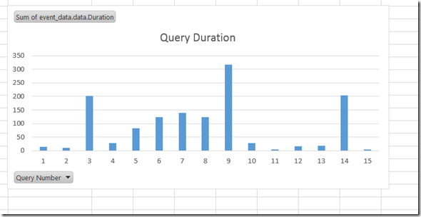
At this point there’s plenty of useful information available: a list of events, a start time for each event, a duration for each event, and other columns where error messages, durations, SQL queries and the number of fields returned by each SQL query. All very useful information when you’re trying to work out why your Power Query query is slow or why it’s not working properly. It’s a shame there isn’t any documentation on what’s in the trace file but as I said, it’s not really for our benefit so I can understand why.

image

At this point you’re on your own, I’m afraid. Happy exploring!


Viewing Error Messages For All Rows In Power Query

$
0
0

One of the great features of Power Query is the way you can view any rows that contain error values when you load data. However, even if you can see the rows that have errors you can’t see the error messages easily – without writing a little bit of M code, which I’ll show you in this post.

Imagine you have the following table of data:

image

…and you load it into Power Query using the following query, which sets the data type for the Sales column to be Whole Number:

let
    Source = Excel.CurrentWorkbook(){[Name="Sales"]}[Content],
    #"Changed Type" = Table.TransformColumnTypes(
                                      Source,
                                     {{"Sales", Int64.Type},
                                      {"Product", type text}})
in
    #"Changed Type"


As you’d expect, the last two rows contain error values as a result of this type conversion:

image

You can also see the number of rows that contain errors when you load the query:

image

Clicking on the “2 errors” link in the screenshot above creates a new query that only contains the rows with errors:

image

You can click on the Error link in any cell that contains one to see the error message:

image

But what you really want is to see the error message for each row. To do this add a new custom column with the following definition:

try [Sales]

image

You will then see a new column called Custom containing a value of type Record. You can then click the Expand icon in the column header (highlighted) and then OK:

image

You’ll then see another column called Custom.Error with an Expand icon; click on it and then click OK again.

image

image

And at last you’ll have two columns that show the error messages for each row:

image


Multiselect, Filtering And Functions In Power Query

$
0
0

If you’re a Power Query enthusiast you’re probably already comfortable with creating functions and passing values to them. However in some scenarios you don’t want to pass just a single value to a parameter, you want to pass multiple values – for example if you are filtering a table by multiple criteria. What’s the best way of handling this in Power Query?

Imagine that you wanted to import data from the DimDate table in the SQL Server Adventure Works DW database. It’s a pretty straightforward date dimension table as you can see:

image

Imagine also that you didn’t want to import all the rows from the table but just those for certain days of the week that the user selects (filtering on the EnglishDayNameOfWeek column).

The first problem is, then, how do you allow the user to make this selection in a friendly way? I’ve already blogged about how the function parameter dialog can be made to show ‘allowed’ selections (here and here) but this only allows selection of single values. One solution I’ve used is to create an Excel table – sourced from a Power Query query of course – and then let users select from there.

In this case, the following query can be used to get all the distinct day names:

let
    Source = Sql.Database("localhost", "adventure works dw"),
    dbo_DimDate = Source{[Schema="dbo",Item="DimDate"]}[Data],
    #"Removed Other Columns" = Table.SelectColumns(dbo_DimDate,
																							{"DayNumberOfWeek", "EnglishDayNameOfWeek"}),
    #"Sorted Rows" = Table.Sort(#"Removed Other Columns",
                                    {{"DayNumberOfWeek", Order.Ascending}}),
    #"Removed Duplicates" = Table.Distinct(#"Sorted Rows"),
    #"Removed Columns" = Table.RemoveColumns(#"Removed Duplicates",
																			{"DayNumberOfWeek"}),
    #"Added Custom" = Table.AddColumn(#"Removed Columns", "Selected", each "No")
in
    #"Added Custom"

Nothing much interesting to say about this apart from that it was all created in the UI, it shows the day names in the correct order, and it has an extra column called Selected that always contains the value “No”. The output table in Excel looks like this:

image

The Selected column is going to allow the end user to choose which days of the week they want to filter the main table by. Since “Yes” and “No” are going to be the only valid values in this column you can use Excel’s Data Validation functionality to show a dropdown box in all of the cells in this column that allows the user from selecting one of those two values and nothing else.

image

image

Once the user has selected “Yes” against all of the day names they want to filter by in the Excel table, the next step is to use this table as the source for another Power Query query. To be clear, we’ve used Power Query to load a table containing day names into an Excel table, where the user can select which days they want to filter by, and we then load this data back into Power Query. This second query (called SelectedDays in this example) then just needs to filter the table so it only returns the rows where Selected is “Yes” and then removes the Selected column once it has done that:

let
    Source = Excel.CurrentWorkbook(){[Name="DistinctDates"]}[Content],
    #"Filtered Rows" = Table.SelectRows(Source, each ([Selected] = "Yes")),
    #"Removed Columns" = Table.RemoveColumns(#"Filtered Rows",{"Selected"})
in
    #"Removed Columns"

image

This query doesn’t need to be loaded anywhere – but it will be referenced later.

With that done, you need to create a function to filter the DimDate table. Here’s the M code:

(SelectedDays as list) =>
let
    Source = Sql.Database("localhost", "adventure works dw"),
    dbo_DimDate = Source{[Schema="dbo",Item="DimDate"]}[Data],
    #"Filtered Rows" = Table.SelectRows(dbo_DimDate,
                             each List.Contains(SelectedDays,[EnglishDayNameOfWeek]) )
in
    #"Filtered Rows"

The thing to notice here is the condition used in the Table.SelectRows() function, where List.Contains() is used to check whether the day name of the current row is present in the list passed in through the SelectedDays parameter.

The final step is to invoke this function and pass the column from the query containing the selected days to it. There is a bit of UI sugar when you invoke a function with a parameter of type list that I blogged about recently. In this case when you invoke the function you just have to pass the pass it the EnglishDayNameOfWeek column from the SelectedDays query.

image

Here’s what the code for the query that invokes the function looks like:

let
    Source = DimDate(SelectedDays[EnglishDayNameOfWeek])
in
    Source

And of course, when you run the query and output the results to a table, you get the DimDate table filtered by all of the days of the week you have selected:

image

To change the output the user just needs to change the selected days and then refresh this last query.

In case you’re wondering, this query does get folded back to SQL Server too. Here’s the SQL generated by Power Query:

select [$Ordered].[DateKey],
    [$Ordered].[FullDateAlternateKey],
    [$Ordered].[DayNumberOfWeek],
    [$Ordered].[EnglishDayNameOfWeek],
    [$Ordered].[SpanishDayNameOfWeek],
    [$Ordered].[FrenchDayNameOfWeek],
    [$Ordered].[DayNumberOfMonth],
    [$Ordered].[DayNumberOfYear],
    [$Ordered].[WeekNumberOfYear],
    [$Ordered].[EnglishMonthName],
    [$Ordered].[SpanishMonthName],
    [$Ordered].[FrenchMonthName],
    [$Ordered].[MonthNumberOfYear],
    [$Ordered].[CalendarQuarter],
    [$Ordered].[CalendarYear],
    [$Ordered].[CalendarSemester],
    [$Ordered].[FiscalQuarter],
    [$Ordered].[FiscalYear],
    [$Ordered].[FiscalSemester]
from
(
    select [_].[DateKey],
        [_].[FullDateAlternateKey],
        [_].[DayNumberOfWeek],
        [_].[EnglishDayNameOfWeek],
        [_].[SpanishDayNameOfWeek],
        [_].[FrenchDayNameOfWeek],
        [_].[DayNumberOfMonth],
        [_].[DayNumberOfYear],
        [_].[WeekNumberOfYear],
        [_].[EnglishMonthName],
        [_].[SpanishMonthName],
        [_].[FrenchMonthName],
        [_].[MonthNumberOfYear],
        [_].[CalendarQuarter],
        [_].[CalendarYear],
        [_].[CalendarSemester],
        [_].[FiscalQuarter],
        [_].[FiscalYear],
        [_].[FiscalSemester]
    from [dbo].[DimDate] as [_]
    where [_].[EnglishDayNameOfWeek] in ('Monday', 'Wednesday', 'Friday')
) as [$Ordered]
order by [$Ordered].[DateKey]

Notice that the Where clause contains an IN condition with all of the selected days.

You can download the example workbook for this post here.


A Closer Look At Power Query/SSAS Integration

$
0
0

In the November release of Power Query the most exciting new feature was the ability to connect to SSAS. I blogged about it at the time, but having used it for a month or so now I thought it was worth writing a more technical post showing how it works in more detail (since some things are not immediately obvious) as well as to see what the MDX it generates looks like.

This post was written using Power Query version 2.18.3874.242, released January 2015; some of the bugs and issues mentioned here will probably be fixed in later versions.

Connecting to SSAS

Power Query officially supports connecting to all versions of SSAS from 2008 onwards, although I’ve heard from a lot of people they have had problems getting the connection working. Certainly when I installed the version of Power Query with SSAS support in on my laptop, which has a full install of SQL Server 2014, it insisted I install the 2012 version of ADOMD.Net before it would work (I also needed to reboot). My guess is that if you’re having problems connecting you should try doing that too; ADOMD.Net 2012 is available to download in the SQL Server 2012 Feature Pack.

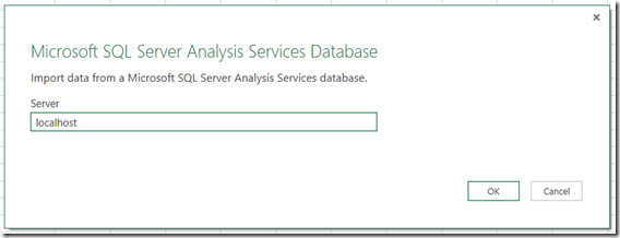
After clicking From Database/From SQL Server Analysis Services the following dialog appears, asking you to enter the name of the server you want to connect to.

image

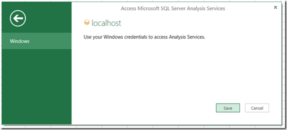
If this is the first time you’re connecting to SSAS the following dialog will appear, asking you to confirm that you want to use Windows credentials to connect.

image

Unfortunately, if you’re connecting via http and need to enter a username and password you won’t be able to proceed any further. I expect this problem will be fixed soon.

Initial Selection

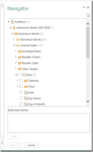
Once you’ve connected the Navigator pane appears on the right-hand side of the screen. Here you see all of the databases on the server you’ve connected to; expand a database and you see the cubes, and within each cube you see all of the measure groups, measures, dimensions and hierarchies.

image

The previous build of Power Query does not display any calculated measures that aren’t associated with measure groups (using the associated_measure_group property); this has been fixed in version 2.18.3874.242.

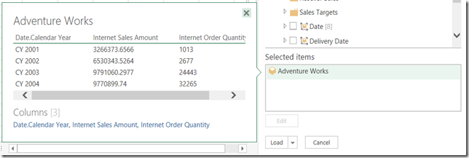
When you start to select measures and hierarchies the name of the cubes you have chosen items from will appear in the Selected items box. If you hover over the name of the cube the peek pane will appear and you’ll see a preview of the results of the query.

image

At this point you can either click the Load button to load the data either to the worksheet or the Excel Data Model, or click the Edit button to edit the query further.

You cannot specify your own MDX query to use for the query as yet.

The Query Editor

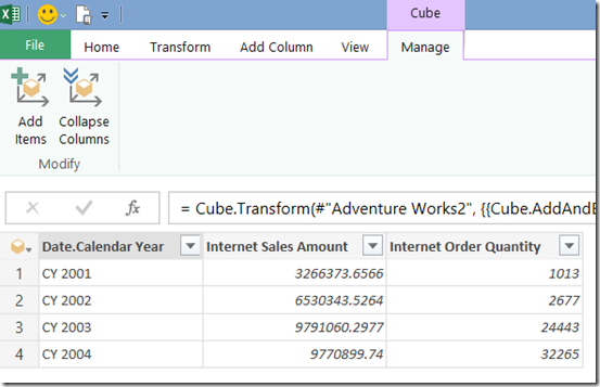
Once the Power Query Query Editor opens you’ll see the output of the query as it stands, and also on the Cube tab in the ribbon two new buttons: Add Items and Collapse Columns.

image

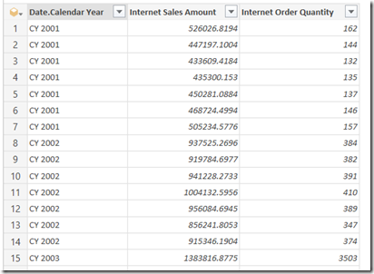
Here’s the MDX (captured from Profiler) showing the MDX generated for the query in the screenshot above:

select
{[Measures].[Internet Sales Amount],[Measures].[Internet Order Quantity]}
on 0,
subset(
nonempty(
[Date].[Calendar Year].[Calendar Year].allmembers
,{[Measures].[Internet Sales Amount],[Measures].[Internet Order Quantity]})
,0,50)
properties member_caption,member_unique_name
on 1
from [Adventure Works]


The MDX Subset() function is used here to ensure that the query doesn’t return more than 50 rows.

Adding Items

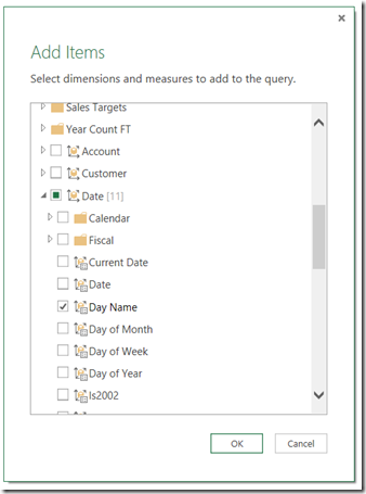
Clicking on the Add Items button allows you to add extra hierarchies and measures to the query. When you click the button the following dialog appears where you can choose what you want to add:

image

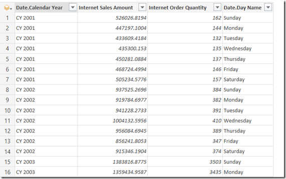
In this case I’ve added the Day Name hierarchy to the query, and this hierarchy appears as a new column on the right-hand edge of the query after the measures:

image

You can easily drag the column to wherever you want it though.

Here’s the MDX again:

select
{[Measures].[Internet Sales Amount],[Measures].[Internet Order Quantity]}
on 0,
subset(
nonempty(
crossjoin(
[Date].[Calendar Year].[Calendar Year].allmembers,
[Date].[Day Name].[Day Name].allmembers)
,{[Measures].[Internet Sales Amount],[Measures].[Internet Order Quantity]})
,0,50)
properties member_caption,member_unique_name
on 1
from [Adventure Works]


Collapsing Columns

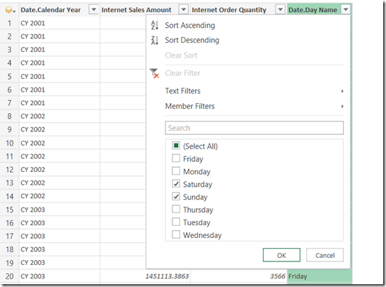
Selecting the Day Name column and then clicking the Collapse Columns button simply rolls back to the previous state of the query. However, there’s more to this button than meets the eye. If you filter the Day Name column (for example, by selecting Saturday and Sunday as in the screenshot below) and then click Collapse and Remove, the filter will still be applied to the query even though the Day Name column is no longer visible.

image

Here’s what the Query Editor shows after the filter and after the Day Name column has been collapsed:

image

Compare the measure values with those shown in the original query – it’s now showing values only for Saturdays and Sundays, although that’s not really clear from the UI. Here’s the MDX generated to prove it – note the use of the subselect to do the filtering:

select
{[Measures].[Internet Sales Amount],[Measures].[Internet Order Quantity]}
on 0,
subset(
nonempty(
[Date].[Calendar Year].[Calendar Year].allmembers
,{[Measures].[Internet Sales Amount],[Measures].[Internet Order Quantity]})
,0,1000)
properties member_caption,member_unique_name
on 1
from(
select
({[Date].[Day Name].&[7],[Date].[Day Name].&[1]})
on 0
from
[Adventure Works])


From studying the MDX generated I can tell that certain other operations such as sorting and filtering the top n rows are folded back to SSAS.

It’s also important to realise that using the Remove option to remove a column from the query does not have the same effect as collapsing the column:

image

Using Remove just hides the column; the number of rows returned by the query remains the same.

image

User Hierarchies

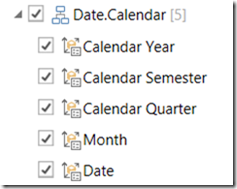
In the examples above I’ve only used attribute hierarchies. User hierarchies aren’t much different – you can select either an individual level or the entire hierarchy (which is the same as selecting all of the levels of the hierarchy).

image

image

Parent-Child Hierarchies

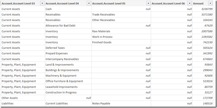
Parent-child hierarchies work very much like user hierarchies, except that you will see some null values in columns to accommodate leaf members at different levels:

image

M Functions

There are a lot of M functions relating to cube functionality, although the documentation in the Library Specification document is fairly basic and all mention of them disappeared from the online help a month or so ago for some reason. Here’s the code for the query in the Collapsing Columns section above:

let
    Source = AnalysisServices.Databases("localhost"),
    #"Adventure Works DW 2008" = Source{[Name="Adventure Works DW 2008"]}[Data],
    #"Adventure Works1" = #"Adventure Works DW 2008"{[Id="Adventure Works"]}[Data],
    #"Adventure Works2" = #"Adventure Works1"{[Id="Adventure Works"]}[Data],
    #"Added Items" = Cube.Transform(#"Adventure Works2", {
             {Cube.AddAndExpandDimensionColumn,
             "[Date]", {"[Date].[Calendar Year].[Calendar Year]"}, {"Date.Calendar Year"}},
             {Cube.AddMeasureColumn, "Internet Sales Amount",
             "[Measures].[Internet Sales Amount]"},
             {Cube.AddMeasureColumn, "Internet Order Quantity",
             "[Measures].[Internet Order Quantity]"}}),
    #"Added Items1" = Cube.Transform(#"Added Items", {
              {Cube.AddAndExpandDimensionColumn, "[Date]",
             {"[Date].[Day Name].[Day Name]"}, {"Date.Day Name"}}}),
    #"Filtered Rows" = Table.SelectRows(#"Added Items1", each (
             Cube.AttributeMemberId([Date.Day Name]) = "[Date].[Day Name].&[7]"
             meta [DisplayName = "Saturday"]
             or
             Cube.AttributeMemberId([Date.Day Name]) = "[Date].[Day Name].&[1]"
             meta [DisplayName = "Sunday"])),
    #"Collapsed and Removed Columns" = Cube.CollapseAndRemoveColumns(
             #"Filtered Rows",
             {"Date.Day Name"})
in
    #"Collapsed and Removed Columns"

It’s comprehensible but not exactly simple – yet another example of how difficult it is to shoe-horn multidimensional concepts into a tool that expects to work with relational data (see also SSRS). I doubt I’ll be writing any M code that uses these functions manually.


Rendering Images In An Excel Worksheet With Power Query Using Cells As Pixels

$
0
0

It’s a general rule of the internet that, whenever you have a cool idea, a few minutes spent on your favourite search engine reveals that someone else has had the idea before you. In my case, when I first saw the functionality in Power Query for working with binary files I wondered whether it was possible to read the contents of a file containing an image and render each pixel as a cell in a worksheet – and of course, it has already been done and done better than I could ever manage. However, it hasn’t been done in Power Query… until now.

First of all, I have to acknowledge the help of Matt Masson whose blog post on working with binary data in Power Query provided a number of useful examples. I also found this article on the bmp file format invaluable.

Second, what I’ve done only works with monochrome bmp files. I could have spent a few more hours coming up with the code to work with other file types but, frankly, I’m too lazy. I have to do real work too, you know.

So let’s see how this works. Here’s a picture of Fountains Abbey that I took on my phone while on holiday last summer:

FountainsAbbey

I opened it in Paint and saved it as a monochrome bmp file:

FountainsAbbey

Here’s the code for the Power Query query that opens the bmp file and renders the contents in Excel:

let
   //The picture to load
   SourceFilePath="C:\Users\Chris\Pictures\FountainsAbbey.bmp",
   //Or get the path from the output of a query called FileName
   //SourceFilePath=FileName,
   //Load the picture
   SourceFile=File.Contents(SourceFilePath),

   //First divide the file contents into two chunks:
   //the header of the file, always 62 bytes
   //and the rest, which contains the pixels

   //Define the format as a record
   OverallFormat=BinaryFormat.Record([
    Header = BinaryFormat.Binary(62),
    Pixels = BinaryFormat.Binary()
    ]),
   //Load the data into that format
   Overall = OverallFormat(SourceFile),
   //Get the header data
   HeaderData = Overall[Header],

   //Extract the total file size and
   //width and height of the image
   HeaderFormat = BinaryFormat.Record([
    Junk1 = BinaryFormat.Binary(2),
    FileSize = BinaryFormat.ByteOrder(
     BinaryFormat.SignedInteger32,
     ByteOrder.LittleEndian),
    Junk2 = BinaryFormat.Binary(12),
    Width = BinaryFormat.ByteOrder(
     BinaryFormat.SignedInteger32,
     ByteOrder.LittleEndian),
    Height = BinaryFormat.ByteOrder(
     BinaryFormat.SignedInteger32,
     ByteOrder.LittleEndian),
    Junk3 = BinaryFormat.Binary()
    ]),
   HeaderValues = HeaderFormat(HeaderData),
   FileSize = HeaderValues[FileSize],
   ImageWidth = HeaderValues[Width],
   ImageHeight = HeaderValues[Height],

   //Each pixel is represented as a bit
   //And each line is made up of groups of four bytes
   BytesPerLine = Number.RoundUp(ImageWidth/32)*4,
   //Read the pixel data into a list
   PixelListFormat = BinaryFormat.List(
    BinaryFormat.ByteOrder(
     BinaryFormat.Binary(BytesPerLine),
     ByteOrder.LittleEndian)),
   PixelList = PixelListFormat(Overall[Pixels]),
   //Convert each byte to a number
   PixelListNumbers = List.Transform(PixelList, each Binary.ToList(_)),

   //A function to convert a number into binary
   //and return a list containing the bits
   GetBinaryNumber = (ValueToConvert as number) as list =>
    let
     BitList = List.Generate(
      ()=>[Counter=1, Value=ValueToConvert],
      each [Counter]<9,
      each [Counter=[Counter]+1,
      Value=Number.IntegerDivide([Value],2)],
      each Number.Mod([Value],2)),
     BitListReversed = List.Reverse(BitList)
    in
     BitListReversed,

   //A function to get all the bits for a single line
   //in the image
   GetAllBitsOnLine = (NumberList as list) =>
    List.FirstN(
     List.Combine(
      List.Transform(NumberList, each GetBinaryNumber(_)
     )
    ), ImageWidth),

   //Reverse the list - the file contains the pixels
   //from the bottom up
   PixelBits = List.Reverse(
    List.Transform(PixelListNumbers,
    each GetAllBitsOnLine(_))),

   //Output all the pixels in a table
   OutputTable = #table(null, PixelBits)
in
    OutputTable


The output of this query is a table containing ones and zeroes and this must be loaded to the worksheet. The final thing to do is to make the table look like a photo by:

  • Hiding the column headers on the table
  • Using the ‘None’ table style so that there is no formatting on the table itself
  • Hiding the values in the table by using the ;;; format (see here for more details)
  • Zooming out as far as you can on the worksheet
  • Resizing the row heights and column widths so the image doesn’t look too squashed
  • Using Excel conditional formatting to make the cells containing 0 black and the cells containing 1 white:image


Here’s the photo rendered as cells in the workbook:

image

And here it is again, zoomed in a bit so you can see the individual cells a bit better:

image

You can download the workbook (which I’ve modified so you can enter the filename of your bmp file in a cell in the worksheet, so you don’t have to edit the query – but you will have to turn Fast Combine on as a result) from here. Have fun!


Expression.Evaluate() In Power Query/M

$
0
0

A year ago I wrote a post on loading the M code for a Power Query query from a text file using the Expression.Evaluate() function, but I admit that at the time I didn’t understand how it worked properly. I’ve now had a chance to look at this function in more detail and thought it might be a good idea to post a few more examples of how it works to add to what’s in the Library spec.

The docs are clear about Expression.Evaluate does: it takes some text containing an M expression and evaluates that expression, returning the result. The important thing to remember here is that an M expression can be more than just a single line of code – a Power Query query is in fact a single expression, and that’s why I was able to execute one using Expression.Evaluate() in the blog post referenced above.

Here’s a simple example of Expression.Evaluate():

let
    Source = Expression.Evaluate("""Hello World""")
in
    Source


It returns, of course, the text “Hello World”:

image

Here’s another example of an expression that returns the number 10:

let
    Source = Expression.Evaluate("6+4")
in
    Source


image

Remember that I said that a Power Query query is itself a single M expression? The way Power Query implements multiple steps in each query is using a let expression, which is a single M expression that contains multiple sub-expressions. Therefore the following  example still shows a single expression (consisting of a let expression) being evaluated to return the value 12:

let
    Source = Expression.Evaluate("let a=3, b=4, c=a*b in c")
in
    Source


image


OK, so far not very interesting. What we really want to do is evaluate more complex M expressions.

Consider the following query, which uses the Text.Upper() function and returns the text ABC:

let
    Source = Text.Upper("abc")
in
    Source


If you run the following query you’ll get the error “The name ‘Text.Upper’ does not exist in the current context.”:

let
    Source = Expression.Evaluate("Text.Upper(""abc"")")
in
    Source

image

To get a full understanding of what’s going on here, I recommend you read section “3.3 Environments and Variables” of the language specification document, which is available here. The short explanation is that all M expressions are evaluated in an ‘environment’, where other variables and functions exist and can be referenced. The reason we’re getting an error in the query above is that it’s trying to execute the expression in an environment all of its own, where the global library functions aren’t available. We can fix this though quite easily by specifying the global environment (where the global library of functions that Text.Upper() is a part of are available) in the second parameter of Expression.Evaluate() using the #shared intrinsic variable, like so:

let
    Source = Expression.Evaluate("Text.Upper(""abc"")", #shared)
in
    Source

image

#shared returns a record containing all of the names of the variables in scope for the global environment and as such it can be used on its own in a query that returns all of the variables (including all of the functions in the global library and from all other queries in the current workbook) available:

let
    Source = #shared
in
    Source


Here’s what that query returns on the workbook that I’m using to write this post, which contains various queries apart from the one above:

image

Reza Rad has a blog post devoted to this which is worth checking out.

Using #shared will allow you to evaluated expressions that use global library functions but it’s not a magic wand that makes all errors go away. The following query declares a list and then attempts to use Expression.Evaluate() to get the second item in the list:

let
    MyList = {1,2,3,4,5},
    GetSecondNumber = Expression.Evaluate("MyList{1}", #shared)
in
    GetSecondNumber

image

Despite the use of #shared in the second parameter we still get the context error we saw before because the variable MyList is still not available. What you need to do here is to define a record in the second parameter of Expression.Evaluate() so that the environment that the expression evaluates in knows what the variable MyList refers to:

let
    MyList = {1,2,3,4,5},
    GetSecondNumber = Expression.Evaluate("MyList{1}", [MyList=MyList])
in
    GetSecondNumber

image

This slightly more complex example, which gets the nth item from a list, might make what’s going on here a little clearer:

let
    MyList_Outer = {1,2,3,4,5},
    NumberToGet_Outer = 3,
    GetNthNumber = Expression.Evaluate("MyList_Inner{NumberToGet_Inner}",
       [MyList_Inner=MyList_Outer, NumberToGet_Inner=NumberToGet_Outer ])
in
    GetNthNumber


image

In this example you can see that the two variable names present in the text passed to the first parameter of Expression.Evaluate() are present in the record used in the second parameter, where they are paired up with the two variables from the main query whose values they use.

Finally, how can you pass your own variable names and use functions from the global library? You need to construct a single record containing all the names in #shared plus any others that you need, and you can do that using Record.Combine() to merge a manually created record with the one returned by #shared as shown here:

let
    MyList_Outer = {1,2,3,4,5},
    NumberToGet_Outer = 1,
    RecordOfVariables =
     [MyList_Inner=MyList_Outer, NumberToGet_Inner=NumberToGet_Outer ],
    RecordOfVariablesAndGlobals = Record.Combine({RecordOfVariables, #shared}),
    GetNthNumber = Expression.Evaluate(
     "List.Reverse(MyList_Inner){NumberToGet_Inner}",
     RecordOfVariablesAndGlobals )
in
    GetNthNumber


image


Handling Added Or Missing Columns In Power Query

$
0
0

A recent conversation in the comments of this blog post brought up the subject of how to handle columns that have either been removed from or added to a data source in Power Query. Anyone who has worked with csv files knows that they have a nasty habit of changing format even when they aren’t supposed to, and added or removed columns can cause all kinds of problems downstream.

Ken Puls (whose excellent blog you are probably already reading if you’re interested in Power Query) pointed out that it’s very easy to protect yourself  against new columns in your data source. When creating a query, select all the columns that you want and then right-click and select Remove Other Columns:

image

This means that if any new columns are added to your data source in the future, they won’t appear in the output of your query. In the M code the Table.SelectColumns() function is used to do this.

Dealing with missing columns is a little bit more complicated. In order to find out whether a column is missing, first of all you’ll need a list of columns that should be present in your query. You can of course store these tables in a table in Excel and enter the column names manually, or you can do this in M fairly easily by creating a query that connects to your data source and using the Table.ColumnNames() function something like this:

let
    //Connect to CSV file
    Source = Csv.Document(
                      File.Contents(
                       "C:\Users\Chris\Documents\Power Query demos\SampleData.csv"
                      ),null,",",null,1252),
    //Use first row as headers
    FirstRowAsHeader = Table.PromoteHeaders(Source),
    //Get a list of column names
    GetColumns = Table.ColumnNames(FirstRowAsHeader),
    //Turn this list into a table
    MakeATable = Table.FromList(
                              GetColumns,
                              Splitter.SplitByNothing(),
                              null,
                              null,
                              ExtraValues.Error),
    //Rename this table's sole column
    RenamedColumns = Table.RenameColumns(
                                         MakeATable ,
                                         {{"Column1", "ColumnName"}})
in
    RenamedColumns

Given a csv file that looks like this:

image

…the query above returns the following table of column names:

image

You can then store the output of this query in an Excel table for future reference – just remember not to refresh the query!

Having done that, you can then look at the columns returned by your data source and compare them with the columns you are expecting by using the techniques shown in this post. For example, here’s a query that reads a list of column names from an Excel table and compares them with the columns returned from a csv file:

let
    //Connect to Excel table containing expected column names
    ExcelSource = Excel.CurrentWorkbook(){[Name="GetColumnNames"]}[Content],
    //Get list of expected columns
    ExpectedColumns = Table.Column(ExcelSource, "ColumnName"),
    //Connect to CSV file
    CSVSource = Csv.Document(
                      File.Contents(
                       "C:\Users\Chris\Documents\Power Query demos\SampleData.csv"
                      ),null,",",null,1252),
    //Use first row as headers
    FirstRowAsHeader = Table.PromoteHeaders(CSVSource),
    //Get a list of column names in csv
    CSVColumns = Table.ColumnNames(FirstRowAsHeader),
    //Find missing columns
    MissingColumns = List.Difference(ExpectedColumns, CSVColumns),
    //Find added columns
    AddedColumns = List.Difference(CSVColumns, ExpectedColumns),
    //Report what has changed
    OutputMissing = if List.Count(MissingColumns)=0 then
                     "No columns missing" else
                     "Missing columns: " & Text.Combine(MissingColumns, ","),
    OutputAdded = if List.Count(AddedColumns)=0 then
                     "No columns added" else
                     "Added columns: " & Text.Combine(AddedColumns, ","),
    Output = OutputMissing & "   " & OutputAdded
in
    Output

Given a csv file that looks like this:

image

…and an Excel table like the one above containing the three column names Month, Product and Sales, the output of this query is:

image

It would be very easy to convert this query to a function that you could use to check the columns expected by multiple queries, and also to adapt the output to your own needs. Also, in certain scenarios (such as when you’re importing data from SQL Server) you might also want to check the data types used by the columns; I’ll leave that for another blog post though. In any case, data types aren’t so much of an issue with CSV files because it’s Power Query that imposes the types on the columns within a query, and any type conversion issues can be dealt with by Power Query’s error handling functionality (see Gerhard Brueckl’s post on this topic, for example).

You can download a workbook containing the two queries from this post here.


Using Excel Slicers To Pass Parameters To Power Query Queries

$
0
0

Power Query is great for filtering data before it gets loaded into Excel, and when you do that you often need to provide a friendly way for end users to choose what data gets loaded exactly. I showed a number of different techniques for doing this last week at SQLBits but here’s my favourite: using Excel slicers.

Using the Adventure Works DW database in SQL Server as an example, imagine you wanted to load only only rows for a particular date or set of dates from the FactInternetSales table. The first step to doing this is to create a query that gets all of the data from the DimDate table (the date dimension you want to use for the filtering). Here’s the code for that query – there’s nothing interesting happening here, all I’m doing is removing unnecessary columns and renaming those that are left:

let
    Source = Sql.Database("localhost", "adventure works dw"),
    dbo_DimDate = Source{[Schema="dbo",Item="DimDate"]}[Data],
    #"Removed Other Columns" = Table.SelectColumns(dbo_DimDate,
        {"DateKey", "FullDateAlternateKey", "EnglishDayNameOfWeek",
        "EnglishMonthName", "CalendarYear"}),
    #"Renamed Columns" = Table.RenameColumns(#"Removed Other Columns",{
        {"FullDateAlternateKey", "Date"}, {"EnglishDayNameOfWeek", "Day"},
        {"EnglishMonthName", "Month"}, {"CalendarYear", "Year"}})
in
    #"Renamed Columns"


Here’s what the output looks like:

image

Call this query Date and then load it to a table on a worksheet. Once you’ve done that you can create Excel slicers on that table (slicers can be created on tables as well as PivotTables in Excel 2013 but not in Excel 2010) by clicking inside it and then clicking the Slicer button on the Insert tab of the Excel ribbon:

image

Creating three slicers on the Day, Month and Year columns allows you to filter the table like so:

image

The idea here is to use the filtered rows from this table as parameters to control what is loaded from the FactInternetSales table. However, if you try to use Power Query to load data from an Excel table that has any kind of filter applied to it, you’ll find that you get all of the rows from that table. Luckily there is a way to determine whether a row in a table is visible or not and I found it in this article written by Excel MVP Charley Kyd:

http://www.exceluser.com/formulas/visible-column-in-excel-tables.htm

You have to create a new calculated column on the table in the worksheet with the following formula:

=(AGGREGATE(3,5,[@DateKey])>0)+0

image

This calculated column returns 1 on a row when it is visible, 0 when it is hidden by a filter. You can then load the table back into Power Query, and when you do you can then filter the table in your new query so that it only returns the rows where the Visible column contains 1 – that’s to say, the rows that are visible in Excel. Here’s the code for this second query, called SelectedDates:

let
    Source = Excel.CurrentWorkbook(){[Name="Date"]}[Content],
    #"Filtered Rows" = Table.SelectRows(Source, each ([Visible] = 1)),
    #"Removed Columns" = Table.RemoveColumns(#"Filtered Rows",{"Visible"})
in
    #"Removed Columns"


image

This query should not be loaded to the Excel Data Model or to the worksheet.

Next, you must use this table to filter the data from the FactInternetSales table. Here’s the code for a query that does that:

let
    Source = Sql.Database("localhost", "adventure works dw"),
    dbo_FactInternetSales = Source{[Schema="dbo",Item="FactInternetSales"]}[Data],
    #"Removed Other Columns" = Table.SelectColumns(dbo_FactInternetSales,
        {"ProductKey", "OrderDateKey", "CustomerKey", "SalesOrderNumber",
        "SalesOrderLineNumber", "SalesAmount", "TaxAmt"}),
    Merge = Table.NestedJoin(#"Removed Other Columns",{"OrderDateKey"},
        SelectedDates,{"DateKey"},"NewColumn",JoinKind.Inner),
    #"Removed Columns" = Table.RemoveColumns(Merge,
        {"ProductKey", "OrderDateKey", "CustomerKey"}),
    #"Expand NewColumn" = Table.ExpandTableColumn(#"Removed Columns",
        "NewColumn", {"Date"}, {"Date"}),
    #"Reordered Columns" = Table.ReorderColumns(#"Expand NewColumn",
        {"Date", "SalesOrderNumber", "SalesOrderLineNumber",
        "SalesAmount", "TaxAmt"}),
    #"Renamed Columns" = Table.RenameColumns(#"Reordered Columns",{
        {"SalesOrderNumber", "Sales Order Number"},
        {"SalesOrderLineNumber", "Sales Order Line Number"},
        {"SalesAmount", "Sales Amount"},
        {"TaxAmt", "Tax Amount"}}),
    #"Changed Type" = Table.TransformColumnTypes(#"Renamed Columns",
        {{"Date", type date}})
in
    #"Changed Type"


Again, most of what this query does is fairly straightforward: removing and renaming columns. The important step where the filtering takes place is called Merge, and here the data from FactInternetSales is joined to the table returned by the SelectedDates query using an inline merge (see here for more details on how to do this):

image

The output of this query is a table containing rows filtered by the dates selected by the user in the slicers, which can then be loaded to a worksheet:

image

The last thing to do is to cut the slicers from the worksheet containing the Date table and paste them onto the worksheet containing the Internet Sales table:

image

You now have a query that displays rows from the FactInternetSales table that are filtered according to the selection made in the slicers. It would be nice if Power Query supported using slicers as a data source direct without using this workaround and you can vote for it to be implemented here.

You can download the sample workbook for this post here.


What’s New In The Excel 2016 Preview For BI?

$
0
0

Following on from my recent post on Power BI and Excel 2016 news, here are some more details about the new BI-related features in the Excel 2016 Preview. Remember that more BI-related features may appear before the release of Excel 2016, and that with Office 365 click-to-run significant new features can appear in between releases, so this is not a definitive list of what Excel 2016 will be able to do at RTM but a snapshot of functionality available as of March 2015 as outlined in this document and which I’ve found from my own investigations. When I find out more, or when new functionality appears, I’ll either update this post or write a new one.

Power Query

Yesterday, in the original version of my post, I mistakenly said that Power Query was a native add-in in Excel 2016: that’s not true, it’s not an add-in at all, it’s native Excel functionality. Indeed you can see that there is no separate Power Query tab any more, and instead there is a Power Query section on the Data tab instead:

DataTab

Obviously I’m a massive fan of Power Query so I’m biased, but I think this is a great move because it makes all the great Power Query functionality a lot easier to discover. There’s nothing to enable – it’s there by default – although I am a bit worried that users will be confused by having the older Data tab features next to their Power Query equivalents.

There are no new features for Power Query here compared to the latest version for Excel 2013, but that’s what I expected.

Excel Forecasting Functions

I don’t pretend to know anything about forecasting, but I had a brief play with the new Forecast.ETS function and got some reasonable results out of it as seen in the screenshot below:

image

Slicer Multiselect

There’s a new hammer icon on a slicer, which, when you click it, changes the way selection works. The default behaviour is the same as Excel 2013: every time you click on an item, that item is selected and any previous selection is lost (unless you were holding control or shift to multiselect). However with the hammer icon selected each new click adds the item to the previously selected items. This is meant to make slicers easier to use with a touch-screen.

Slicer

Time Grouping in PivotTables

Quite a neat feature this, I think. If you have a table in the Excel Data Model that has a column of type date in it, you can add extra calculated columns to that table from within a PivotTable to group by things like Year and Month. For example, here’s a PivotTable I built on a table that contains just dates:

Group1

Right-clicking on the field containing the dates and clicking Group brings up the following dialog:

Group2

Choosing Years, Quarters and Months creates three extra fields in the PivotTable:

Group3

And these fields are implemented as calculated columns in the original table in the Excel Data Model, with DAX definitions as seen here:

Group4

Power View on SSAS Multidimensional

At-bloody-last. I haven’t installed SSAS on the VM I’m using for testing Excel 2016, but I assume it just works. Nothing new in Power View yet, by the way.

Power Map data cards

Not sure why this is listed as new in Excel 2016 when it seems to be the same feature that appeared in Excel 2013 Power Map recently:

https://support.office.com/en-za/article/Customize-a-data-card-in-Power-Map-797ab684-82e0-4705-a97f-407e4a576c6e

Power Pivot

There isn’t any obvious new functionality in the Power Pivot window, but it’s clear that the UI in general and the DAX formula editor experience in particular has been improved.

image

Suggested Relationships

When you use fields from two Excel Data Model tables that have no relationship between them in a PivotTable, you get a prompt to either create new relationships yourself or let Excel detect the relationships:

image

Renaming Tables and Fields in the Power Pivot window

In Excel 2013 when you renamed tables or fields in the Excel Data Model, any PivotTables that used those objects had them deleted. Now, in Excel 2016, the PivotTable retains the reference to table or field and just displays the new name. What’s even better is that when you create a measure or a calculated column that refers to a table or column, the DAX definition of the measure or calculated column gets updated after a rename too.

DAX

There are lots of new DAX functions in this build. With the help of the mdschema_functions schema rowset and Power Query I was able to compare the list of DAX functions available in 2016 with those in 2013 and create the following list of new DAX functions and descriptions:

FUNCTION NAME		DESCRIPTION
DATEDIFF			Returns the number of units (unit specified in Interval)
			between the input two dates
CONCATENATEX		Evaluates expression for each row on the table, then
			return the concatenation of those values in a single string
			result, separated by the specified delimiter
KEYWORDMATCH		Returns TRUE if there is a match between the
			MatchExpression and Text.
ADDMISSINGITEMS		Add the rows with empty measure values back.
CALENDAR			Returns a table with one column of all dates between
			StartDate and EndDate
CALENDARAUTO		Returns a table with one column of dates
			calculated from the model automatically
CROSSFILTER		Specifies cross filtering direction to be used in
			the evaluation of a DAX expression. The relationship is
			defined by naming, as arguments, the two columns that
			serve as endpoints
CURRENTGROUP		Access to the (sub)table representing current
			group in GroupBy function. Can be used only inside GroupBy
			function.
GROUPBY			Creates a summary the input table grouped by the
			specified columns
IGNORE			Tags a measure expression specified in the call to
			SUMMARIZECOLUMNS function to be ignored when
			determining the non-blank rows.
ISONORAFTER		The IsOnOrAfter function is a boolean function that
			emulates the behavior of Start At clause and returns
			true for a row that meets all the conditions mentioned as
			parameters in this function.
NATURALINNERJOIN		Joins the Left table with right table using the
			Inner Join semantics
NATURALLEFTOUTERJOIN	Joins the Left table with right table
			using the Left Outer Join semantics
ROLLUPADDISSUBTOTAL		Identifies a subset of columns specified
			in the call to SUMMARIZECOLUMNS function that should be
			used to calculate groups of subtotals
ROLLUPISSUBTOTAL		Pairs up the rollup groups with the column
			added by ROLLUPADDISSUBTOTAL
SELECTCOLUMNS		Returns a table with selected columns from the table
			and new columns specified by the DAX expressions
SUBSTITUTEWITHINDEX		Returns a table which represents the semijoin of two
			tables supplied and for which the common set of
			columns are replaced by a 0-based index column.
			The index is based on the rows of the second table
			sorted by specified order expressions.
SUMMARIZECOLUMNS		Create a summary table for the requested
			totals over set of groups.
GEOMEAN			Returns geometric mean of given column
			reference.
GEOMEANX			Returns geometric mean of an expression
			values in a table.
MEDIANX			Returns the 50th percentile of an expression
			values in a table.
PERCENTILE.EXC		Returns the k-th (exclusive) percentile of
			values in a column.
PERCENTILE.INC		Returns the k-th (inclusive) percentile of
			values in a column.
PERCENTILEX.EXC		Returns the k-th (exclusive) percentile of an
			expression values in a table.
PERCENTILEX.INC		Returns the k-th (inclusive) percentile of an
			expression values in a table.
PRODUCT			Returns the product of given column reference.
PRODUCTX			Returns the product of an expression
			values in a table.
XIRR			Returns the internal rate of return for a schedule of
			cash flows that is not necessarily periodic
XNPV			Returns the net present value for a schedule of cash flows

Plenty of material for future blog posts there, I think – there are lots of functions here that will be very useful. I bet Marco and Alberto are excited…

VBA

It looks like we have support for the Excel Data Model (aka Power Pivot) in VBA at last.

VBAModel

I need to do some research here, but I get the distinct feeling that the only things that are possible through VBA are the things you can do in the Excel ribbon, such as creating connections, tables and relationships. I can’t see any support for creating measures, calculated columns or hierarchies…? I can’t see anything relating to Power Query either. Maybe I’m not looking in the right place; maybe something will come in a later build?

UPDATE: I’m an idiot – there is one minor change to the VBA support for the Excel Data Model, but actually almost everything that I see in 2016 is also present in 2013. Sorry…


Benford’s Law And Power Query

$
0
0

Probably my favourite session at SQLBits the other week was Professor Mark Whitehorn on exploiting exotic patterns in data. One of the things he talked about was Benford’s Law, something I first heard about several years ago (in fact I’m sure I wrote a blog post on implementing Benford’s Law in MDX but I can’t find it), about the frequency distribution of digits in data. I won’t try to explain it myself but there are plenty of places you can read up on it, for example: http://en.wikipedia.org/wiki/Benford%27s_law . I promise, it’s a lot more interesting that it sounds!

Anyway, it struck me that it would be quite useful to have a Power Query function that could be used to find the distribution of the first digits in any list of numbers, for example for fraud detection purposes. The first thing I did was write a simple query that returned the expected distributions for the digits 1 to 9 according to Benford’s Law:

let
    //function to find the expected distribution of any given digit
    Benford = (digit as number) as number => Number.Log10(1 + (1/digit)),
    //get a list of values between 1 and 9
    Digits = {1..9},
    // get a list containing these digits and their expected distribution
    DigitsAndDist = List.Transform(Digits, each {_, Benford(_)}),
    //turn that into a table
    Output = #table({"Digit", "Distribution"}, DigitsAndDist)
in
    Output


image

Next I wrote the function itself:

//take a single list of numbers as a parameter
(NumbersToCheck as list) as table=>
let
    //remove any non-numeric values
    RemoveNonNumeric = List.Select(NumbersToCheck,
                        each Value.Is(_, type number)),
    //remove any values that are less than or equal to 0
    GreaterThanZero = List.Select(RemoveNonNumeric, each _>0),
    //turn that list into a table
    ToTable = Table.FromList(GreaterThanZero,
                        Splitter.SplitByNothing(), null, null,
                        ExtraValues.Error),
    RenameColumn = Table.RenameColumns(ToTable,{{"Column1", "Number"}}),
    //function to get the first digit of a number
    FirstDigit = (InputNumber as number) as
                    number =>
                    Number.FromText(Text.Start(Number.ToText(InputNumber),1))-1,
    //get the distributions of each digit
    GetDistributions = Table.Partition(RenameColumn,
                    "Number", 9, FirstDigit),
    //turn that into a table
    DistributionTable = Table.FromList(GetDistributions,
                    Splitter.SplitByNothing(), null, null, ExtraValues.Error),
    //add column giving the digit
    AddIndex = Table.AddIndexColumn(DistributionTable, "Digit", 1, 1),
    //show how many times each first digit occurred
    CountOfDigits = Table.AddColumn(AddIndex,
                    "Count", each Table.RowCount([Column1])),
    RemoveColumn = Table.RemoveColumns(CountOfDigits ,{"Column1"}),
    //merge with table showing expected distributions
    Merge = Table.NestedJoin(RemoveColumn,{"Digit"},
                             Benford,{"Digit"},"NewColumn",JoinKind.Inner),
    ExpandNewColumn = Table.ExpandTableColumn(Merge, "NewColumn",
                            {"Distribution"}, {"Distribution"}),
    RenamedDistColumn = Table.RenameColumns(ExpandNewColumn,
                            {{"Distribution", "Expected Distribution"}}),
    //calculate actual % distribution of first digits
    SumOfCounts = List.Sum(Table.Column(RenamedDistColumn, "Count")),
    AddActualDistribution = Table.AddColumn(RenamedDistColumn,
                            "Actual Distribution", each [Count]/SumOfCounts)
in
    AddActualDistribution

There’s not much to say about this code, apart from the fact that it’s a nice practical use case for the Table.Partition() function I blogged about here. It also references the first query shown above, called Benford, so that the expected and actual distributions can be compared.

Since this is a function that takes a list as a parameter, it’s very easy to pass it any column from any other Power Query query that’s in the same worksheet (as I showed here) for analysis. For example, I created a Power Query query on this dataset in the Azure Marketplace showing the number of minutes that each flight in the US was delayed in January 2012. I then invoked the function above, and pointed it at the column containing the delay values like so:

image

The output is a table (to which I added a column chart) which shows that this data follows the expected distribution very closely:

image

You can download my sample workbook containing all the code from here.


Analysing SSAS Extended Event Data With Power Query: Part 1

$
0
0

The other day, while I was reading this post by Melissa Coates, I was reminded of the existence of extended events in SSAS. I say ‘reminded’ because although this is a subject I’ve blogged about before, I have never done anything serious with extended events because you can get the same data from Profiler much more easily, so I had pretty much forgotten about them. But… while Profiler is good, it’s a long way from perfect and there’s a lot of information that you can get from a trace that is still very hard to analyse. I started thinking: what if there was a tool we could use to analyse the data captured by extended events easily? [Lightbulb moment] Of course, Power Query!

I’m not going to go over how to use Extended Events in SSAS because the following blog posts do a great job already:
http://byobi.com/blog/2013/06/extended-events-for-analysis-services/
http://markvsql.com/2014/02/introduction-to-analysis-services-extended-events/
https://francescodechirico.wordpress.com/2012/08/03/identify-storage-engine-and-formula-engine-bottlenecks-with-new-ssas-xevents-5/

You may also want to check out these (old, but still relevant) articles on performance tuning SSAS taken from the book I co-wrote with Marco and Alberto, “Expert Cube Development”:

http://www.packtpub.com/article/query-performance-tuning-microsoft-analysis-services-part1
http://www.packtpub.com/article/query-performance-tuning-microsoft-analysis-services-part2

What I want to concentrate on in this series of posts is how to make sense of this data using Power BI in general and Power Query in particular. The first step is to be able to load data from the .xel file using Power Query, and that’s what this post will cover. In the future I want to explore how to get at and use specific pieces of text data such as that given by the Query Subcube Verbose, Calculation Evaluation and Resource Usage events, and to show how this data can be used to solve difficult performance problems. I’m only going to talk about SSAS Multidimensional, but of course a lot of what I show will be applicable (or easily adapted to) Tabular; I guess you could also do something similar for SQL Server Extended Events too. I’m also going to focus on ad hoc analysis of this data, rather than building a more generic performance monitoring solution; the latter is a perfectly valid thing to want to build, but why build one yourself when companies like SQL Sentry have great tools for this purpose that you can buy off the shelf?

Anyway, let’s get on. Here’s a Power Query function that can be used to get data from one or more .xel files generated by SSAS:

(servername as text,
initialcatalog as text,
filename as text)
as table =>
let
    //Query the xel data
    Source = Sql.Database(servername,
                          initialcatalog,
                          [Query="SELECT
                          object_name, event_data, file_name
                          FROM sys.fn_xe_file_target_read_file ( '"
                          & filename & "', null, null, null )"]),
    //Treat the contents of the event_data column
    //as XML
    ParseXML = Table.TransformColumns(Source,
                            {{"event_data", Xml.Tables}}),
    //Expand that column
    Expandevent_data = Table.ExpandTableColumn(ParseXML,
                            "event_data",
                            {"Attribute:timestamp", "data"},
                            {"event_data.Attribute:timestamp",
                            "event_data.data"}),
    //A function to tranpose the data held in the
    //eventdata.data column
    GetAttributeData = (AttributeTable as table) as table =>
	let
    	  RemoveTextColumn = Table.RemoveColumns(AttributeTable,
                            {"text"}),
          SetTypes = Table.TransformColumnTypes(RemoveTextColumn ,
                            {{"value", type text}, {"Attribute:name", type text}}),
          TransposeTable = Table.Transpose(SetTypes),
          ReverseRows = Table.ReverseRows(TransposeTable),
          PromoteHeaders = Table.PromoteHeaders(ReverseRows)
	in
          PromoteHeaders,
    //Use the function above
    ParseAttributeData = Table.TransformColumns(Expandevent_data,
                            {"event_data.data", GetAttributeData})
in
    ParseAttributeData


This function can be thought of as the starting point for everything else: it allows you to load the raw data necessary for any SSAS performance tuning work. Its output can then, in turn, be filtered and transformed to solve particular problems.

The function takes three parameters:

  • The name of a SQL Server relational database instance – this is because I’m using sys.fn_exe_file_target_read_file to actually read the data from the .xel file. I guess I could try to parse the binary data in the .xel file, but why make things difficult?
  • The name of a database on that SQL Server instance
  • The file name (including the full path) or pattern for the .xel files

The only other thing to mention here is that the event_data column contains XML data, which of course Power Query can handle quite nicely, but even then the data in the XML needs to be cleaned and transposed before you can get a useful table of data. The GetAttributeData function in the code above does this cleaning and transposing but, when invoked, the function still returns an unexpanded column called event_data.data as seen in the following screenshot:

image

There are two reasons why the function does not expand this column for you:

  1. You probably don’t want to see every column returned by every event
  2. Expanding all the columns in a nested table, when you don’t know what the names of these columns are, is not trivial (although this post shows how to do it)

Here’s an example of how the function can be used:

let
    //Invoke the GetXelData function
    Source = GetXelData(
                        "localhost",
                        "adventure works dW",
                        "C:\SSAS_Monitoring*.xel"),
    //Only return Query End events
    #"Filtered Rows" = Table.SelectRows(Source,
                        each ([object_name] = "QueryEnd")),
    //Expand Duration and TextData columns
    #"Expand event_data.data" = Table.ExpandTableColumn(
                        #"Filtered Rows", "event_data.data",
                        {"Duration", "TextData"},
                        {"event_data.data.Duration",
                        "event_data.data.TextData"}),
    //Set some data types
    #"Changed Type" = Table.TransformColumnTypes(
                        #"Expand event_data.data",
                        {{"event_data.Attribute:timestamp", type datetime},
                        {"event_data.data.Duration", Int64.Type}}),
    //Sort by timestamp
    #"Sorted Rows" = Table.Sort(#"Changed Type",
                        {{"event_data.Attribute:timestamp", Order.Ascending}}),
    //Add an index column to identify each query
    #"Added Index" = Table.AddIndexColumn(#"Sorted Rows", "Query Number", 1, 1),
    //Remove unwanted columns
    #"Removed Columns" = Table.RemoveColumns(#"Added Index",
                        {"object_name", "file_name"})
in
    #"Removed Columns"


All that’s happening here is that the function is being called in the first step, Source, and then I’m filtering by the Query End event, expanding some of the columns in event_data.data and setting column data types. You won’t need to copy all this code yourself though – you just need to invoke the function and then expand the event_data.data column to reveal whatever columns you are interested in. When you run a query that calls this function for the first time, you may need to give Power Query permission to connect to SQL Server and also to run a native database query.

Here’s an example PivotChart showing query durations built from this data after it has been loaded to the Excel Data Model:

image

Not very useful, for sure, but in the next post you’ll see a more practical use for this function.

You can download the sample workbook for this post here.


Building A Reporting Solution Using Power Query

$
0
0

The video of my SQLBits conference session “Building a reporting solution using Power Query” is now available to view (for free) on the SQLBits website:
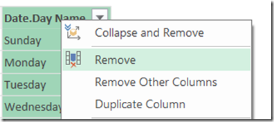
http://sqlbits.com/Sessions/Event14/Building_A_Reporting_Solution_Using_Power_Query

It’s not your normal Power Query session about self-service ETL – instead it’s about using Power Query to create a SSRS-like reporting solution inside Excel. This is a topic I’ve been thinking about for a while, and while I have blogged about some of the tricks I show in the session (like this one about using slicers to pass parameters to Power Query) there’s a lot of new material in there too that should interest all you Power Query fans.

Of course there are literally hundreds of other great videos to watch for free at http://sqlbits.com/content/ including many others on Power BI, Power Pivot and Power Query. Alas my “Amazing Things You Can Do With Power BI” session video hasn’t been posted yet though…

[Don’t forget I’m running public Power BI and Power Query training courses in London next month! Full details at http://technitrain.com/courses.php]


Power Query Announcements At The PASS BA Conference

$
0
0

There were a couple of big (well, big if you’re a Power Query fan like me) announcements made today by Miguel Llopis at the PASS BA Conference:

  • Today Power Query is available only to people who have Excel Professional Plus or Excel standalone, but as of May a version of Power Query will be available on every Excel SKU. There will be some limitations around data sources that are supported if you don’t have Excel Professional Plus, but that’s ok – this change will make it much easier for people to learn about and use Power Query, and I’m really happy about that.
  • Other new features coming in the May update of Power Query include the ability to turn off prompts about native database queries (useful in this scenario, for example), OData v4.0 support, the ability to use alternative Windows credentials to run queries, and a couple of new transformations such as removing empty rows.
  • Excel 2016 – where Power Query is now native to Excel – will have support for creating Power Query queries using VBA and macro recording. I understand you won’t be able to edit individual steps in a query, but you’ll be able to create and delete queries programmatically and change where they load their data too.
  • Excel 2016 will also support undo/redo for Power Query and give you the ability to copy/paste queries (even from workbook to workbook).
  • There was a commitment that Power Query in Excel 2016 will keep getting updates on a regular basis, rather than get tied to the much slower Office release cycle, so it retains parity with the Power Query functionality in the Power BI Dashboard Designer.

All very cool stuff!


Viewing all 252 articles
Browse latest View live


<script src="https://jsc.adskeeper.com/r/s/rssing.com.1596347.js" async> </script>