In the November release of Power Query the most exciting new feature was the ability to connect to SSAS. I blogged about it at the time, but having used it for a month or so now I thought it was worth writing a more technical post showing how it works in more detail (since some things are not immediately obvious) as well as to see what the MDX it generates looks like.
This post was written using Power Query version 2.18.3874.242, released January 2015; some of the bugs and issues mentioned here will probably be fixed in later versions.
Connecting to SSAS
Power Query officially supports connecting to all versions of SSAS from 2008 onwards, although I’ve heard from a lot of people they have had problems getting the connection working. Certainly when I installed the version of Power Query with SSAS support in on my laptop, which has a full install of SQL Server 2014, it insisted I install the 2012 version of ADOMD.Net before it would work (I also needed to reboot). My guess is that if you’re having problems connecting you should try doing that too; ADOMD.Net 2012 is available to download in the SQL Server 2012 Feature Pack.
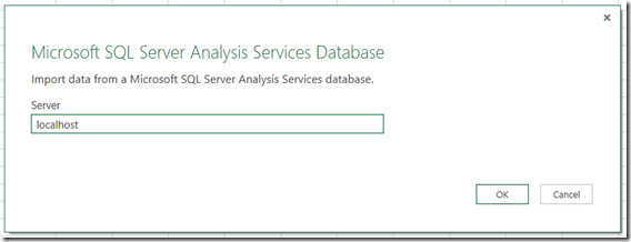
After clicking From Database/From SQL Server Analysis Services the following dialog appears, asking you to enter the name of the server you want to connect to.
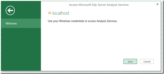
If this is the first time you’re connecting to SSAS the following dialog will appear, asking you to confirm that you want to use Windows credentials to connect.
Unfortunately, if you’re connecting via http and need to enter a username and password you won’t be able to proceed any further. I expect this problem will be fixed soon.
Initial Selection
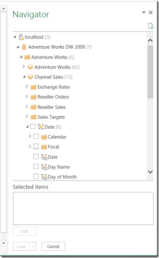
Once you’ve connected the Navigator pane appears on the right-hand side of the screen. Here you see all of the databases on the server you’ve connected to; expand a database and you see the cubes, and within each cube you see all of the measure groups, measures, dimensions and hierarchies.
The previous build of Power Query does not display any calculated measures that aren’t associated with measure groups (using the associated_measure_group property); this has been fixed in version 2.18.3874.242.
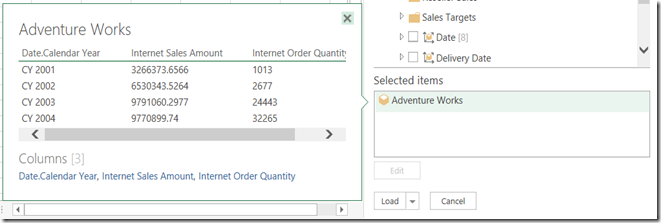
When you start to select measures and hierarchies the name of the cubes you have chosen items from will appear in the Selected items box. If you hover over the name of the cube the peek pane will appear and you’ll see a preview of the results of the query.
At this point you can either click the Load button to load the data either to the worksheet or the Excel Data Model, or click the Edit button to edit the query further.
You cannot specify your own MDX query to use for the query as yet.
The Query Editor
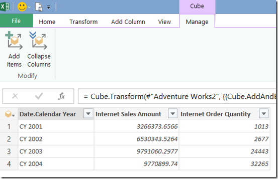
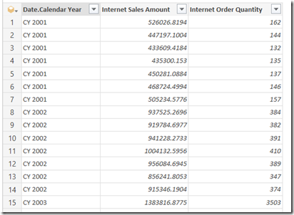
Once the Power Query Query Editor opens you’ll see the output of the query as it stands, and also on the Cube tab in the ribbon two new buttons: Add Items and Collapse Columns.
Here’s the MDX (captured from Profiler) showing the MDX generated for the query in the screenshot above:
select
{[Measures].[Internet Sales Amount],[Measures].[Internet Order Quantity]}
on 0,
subset(
nonempty(
[Date].[Calendar Year].[Calendar Year].allmembers
,{[Measures].[Internet Sales Amount],[Measures].[Internet Order Quantity]})
,0,50)
properties member_caption,member_unique_name
on 1
from [Adventure Works]
The MDX Subset() function is used here to ensure that the query doesn’t return more than 50 rows.
Adding Items
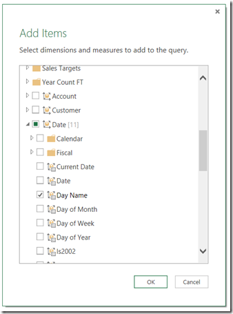
Clicking on the Add Items button allows you to add extra hierarchies and measures to the query. When you click the button the following dialog appears where you can choose what you want to add:
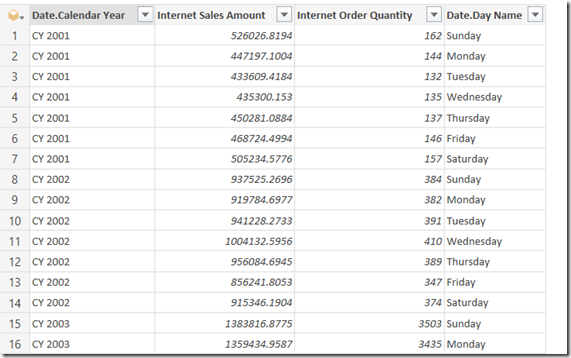
In this case I’ve added the Day Name hierarchy to the query, and this hierarchy appears as a new column on the right-hand edge of the query after the measures:
You can easily drag the column to wherever you want it though.
Here’s the MDX again:
select
{[Measures].[Internet Sales Amount],[Measures].[Internet Order Quantity]}
on 0,
subset(
nonempty(
crossjoin(
[Date].[Calendar Year].[Calendar Year].allmembers,
[Date].[Day Name].[Day Name].allmembers)
,{[Measures].[Internet Sales Amount],[Measures].[Internet Order Quantity]})
,0,50)
properties member_caption,member_unique_name
on 1
from [Adventure Works]
Collapsing Columns
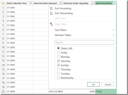
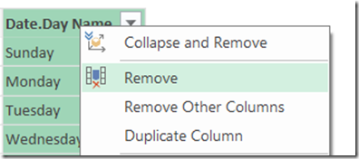
Selecting the Day Name column and then clicking the Collapse Columns button simply rolls back to the previous state of the query. However, there’s more to this button than meets the eye. If you filter the Day Name column (for example, by selecting Saturday and Sunday as in the screenshot below) and then click Collapse and Remove, the filter will still be applied to the query even though the Day Name column is no longer visible.
Here’s what the Query Editor shows after the filter and after the Day Name column has been collapsed:
Compare the measure values with those shown in the original query – it’s now showing values only for Saturdays and Sundays, although that’s not really clear from the UI. Here’s the MDX generated to prove it – note the use of the subselect to do the filtering:
select
{[Measures].[Internet Sales Amount],[Measures].[Internet Order Quantity]}
on 0,
subset(
nonempty(
[Date].[Calendar Year].[Calendar Year].allmembers
,{[Measures].[Internet Sales Amount],[Measures].[Internet Order Quantity]})
,0,1000)
properties member_caption,member_unique_name
on 1
from(
select
({[Date].[Day Name].&[7],[Date].[Day Name].&[1]})
on 0
from
[Adventure Works])
From studying the MDX generated I can tell that certain other operations such as sorting and filtering the top n rows are folded back to SSAS.
It’s also important to realise that using the Remove option to remove a column from the query does not have the same effect as collapsing the column:
Using Remove just hides the column; the number of rows returned by the query remains the same.
User Hierarchies
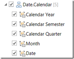
In the examples above I’ve only used attribute hierarchies. User hierarchies aren’t much different – you can select either an individual level or the entire hierarchy (which is the same as selecting all of the levels of the hierarchy).
Parent-Child Hierarchies
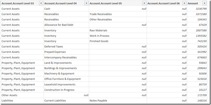
Parent-child hierarchies work very much like user hierarchies, except that you will see some null values in columns to accommodate leaf members at different levels:
M Functions
There are a lot of M functions relating to cube functionality, although the documentation in the Library Specification document is fairly basic and all mention of them disappeared from the online help a month or so ago for some reason. Here’s the code for the query in the Collapsing Columns section above:
let
    Source = AnalysisServices.Databases("localhost"),
    #"Adventure Works DW 2008" = Source{[Name="Adventure Works DW 2008"]}[Data],
    #"Adventure Works1" = #"Adventure Works DW 2008"{[Id="Adventure Works"]}[Data],
    #"Adventure Works2" = #"Adventure Works1"{[Id="Adventure Works"]}[Data],
    #"Added Items" = Cube.Transform(#"Adventure Works2", {
             {Cube.AddAndExpandDimensionColumn,
             "[Date]", {"[Date].[Calendar Year].[Calendar Year]"}, {"Date.Calendar Year"}},
             {Cube.AddMeasureColumn, "Internet Sales Amount",
             "[Measures].[Internet Sales Amount]"},
             {Cube.AddMeasureColumn, "Internet Order Quantity",
             "[Measures].[Internet Order Quantity]"}}),
    #"Added Items1" = Cube.Transform(#"Added Items", {
              {Cube.AddAndExpandDimensionColumn, "[Date]",
             {"[Date].[Day Name].[Day Name]"}, {"Date.Day Name"}}}),
    #"Filtered Rows" = Table.SelectRows(#"Added Items1", each (
             Cube.AttributeMemberId([Date.Day Name]) = "[Date].[Day Name].&[7]"
             meta [DisplayName = "Saturday"]
             or
             Cube.AttributeMemberId([Date.Day Name]) = "[Date].[Day Name].&[1]"
             meta [DisplayName = "Sunday"])),
    #"Collapsed and Removed Columns" = Cube.CollapseAndRemoveColumns(
             #"Filtered Rows",
             {"Date.Day Name"})
in
    #"Collapsed and Removed Columns"
It’s comprehensible but not exactly simple – yet another example of how difficult it is to shoe-horn multidimensional concepts into a tool that expects to work with relational data (see also SSRS). I doubt I’ll be writing any M code that uses these functions manually.
